Nearest Neighbor Indexes for Similarity Search
Vector similarity search is a game-changer in the world of search. It allows us to efficiently search a huge range of media, from GIFs to articles — with incredible accuracy in sub-second timescales for billion+ size datasets.
One of the key components to efficient search is flexibility. And for that we have a wide range of search indexes available to us — there is no ‘one-size-fits-all’ in similarity search.
However, this great flexibility produces a question — how do we know which size fits our use case?
Which index do we choose? Should we use multiple indexes, or is one enough?
This article will explore the pros and cons of some of the most important indexes — Flat, LSH, HNSW, and IVF. We will learn how we decide which to use and the impact of parameters in each index.
Note: Pinecone lets you add vector search to your production applications without knowing anything about vector indexes. However, we know you like seeing how things work, so enjoy learning about these popular vector index types!
Check out the video walkthrough:
Indexes in Search
Before jumping into the different indexes available, let’s take a look at why we care about similarity search — and how we can use indexes for efficient similarity search.
Why Similarity Search
Let’s start with the most fundamental question to the relevance of this article — why do we care about similarity search?
Similarity search can be used to compare data quickly. Given a query (which could be in any format — text, audio, video, GIFs — you name it), we can use similarity search to return relevant results.
This is key to a huge number of companies and applications spanning across industries. It’s used to identify similar genes in genome databases, deduplication of datasets, or search billions of results to search queries every day.
Search seems like an easy process — we take one item and compare it to another. But when we have millions (or even billions) of ‘other’ items to compare against — it begins to get tricky.
For search to be useful, it needs to be accurate and fast. And it is this more efficient search that we are interested in.
Indexes For Efficient Search
In vector similarity search, we use an index to store vector representations of the data we intend to search.
Through either statistical methods or machine learning — we can build vectors that encode useful, meaningful information about our original data.
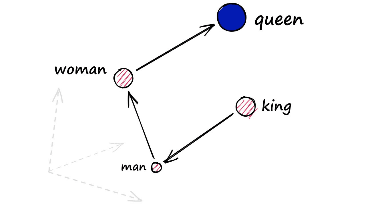
We take these ‘meaningful’ vectors and store them inside an index to use for intelligent similarity search.
There are many index solutions available; one, in particular, is called Faiss (Facebook AI Similarity Search). We store our vectors in Faiss and query our new Faiss index using a ‘query’ vector. This query vector is compared to other index vectors to find the nearest matches — typically with Euclidean (L2) or inner-product (IP) metrics.
So, with that introduction to the why and how of similarity search. But what is this about Faiss — and choosing the right indexes?
Faiss And Indexes
Faiss comes with many different index types — many of which can be mixed and matched to produce multiple layers of indexes.
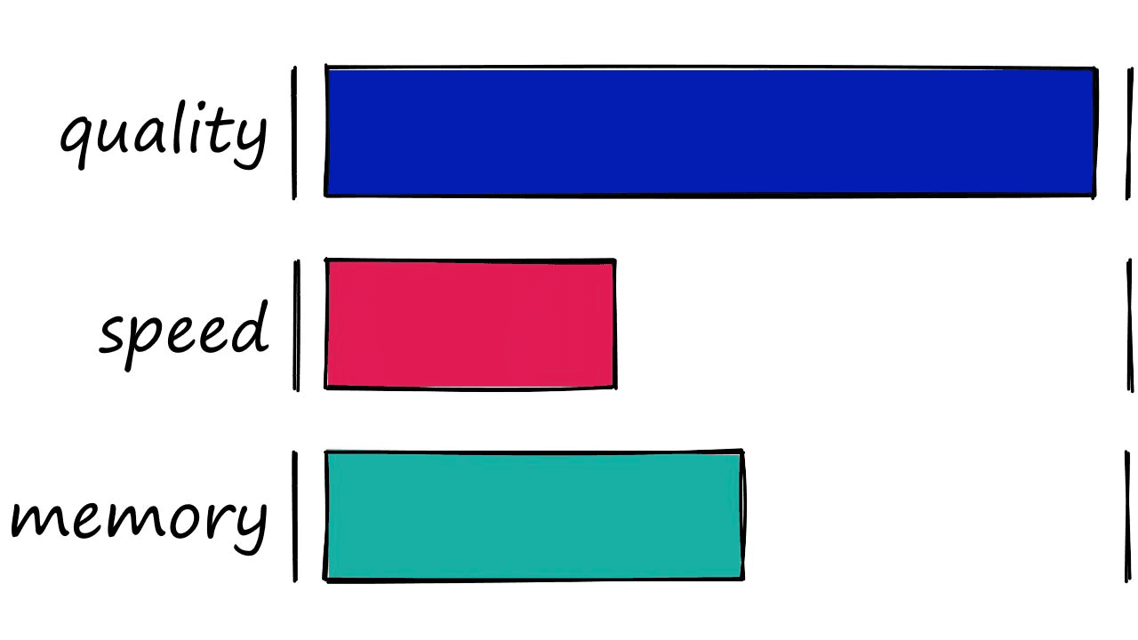
We will be focused on a few indexes that prioritize search speed, quality, or index memory.
Now, which one of these indexes we use depends very much on our use case. We must consider factors such as dataset size, search frequency, or search-quality vs. search-speed.
Flat And Accurate
The very first indexes we should look at are the simplest — flat indexes.
Flat indexes are ‘flat’ because we do not modify the vectors that we feed into them.
Because there is no approximation or clustering of our vectors — these indexes produce the most accurate results. We have perfect search quality, but this comes at the cost of significant search times.
With flat indexes, we introduce our query vector xqand compare it against every other full-size vector in our index — calculating the distance to each.
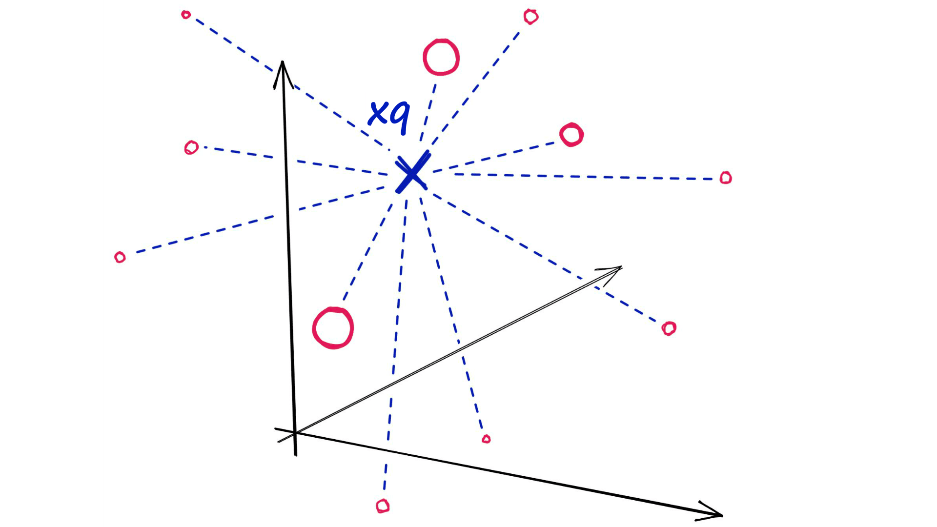
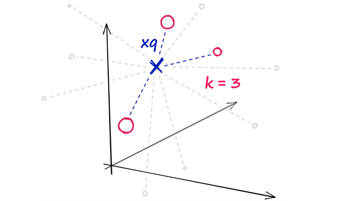
After calculating all of these distances, we will return the nearest k of those as our nearest matches. A k-nearest neighbors (kNN) search.
When To Use
So when should we use a flat index? Well, when search quality is an unquestionably high priority — and search speed is less important.
Search speed can be an irrelevant factor for smaller datasets — especially when using more powerful hardware.
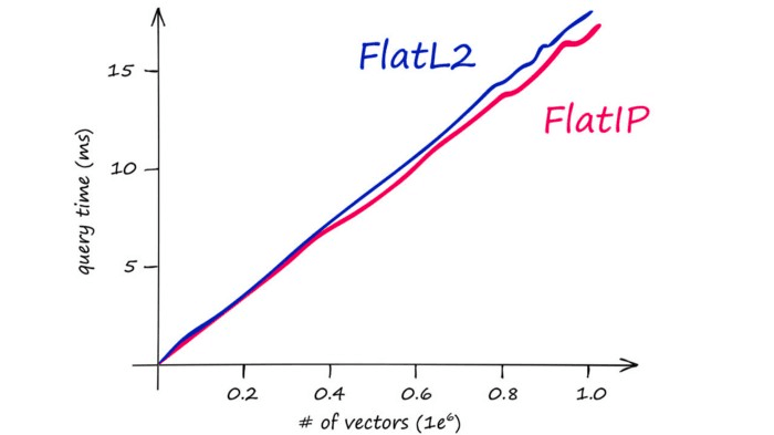
The above chart demonstrates Faiss CPU speeds on an M1-chip. Faiss is optimized to run on GPU at significantly higher speeds when paired with CUDA-enabled GPUs on Linux to improve search times significantly.
In short, use flat indexes when:
- Search quality is a very high priority.
- Search time does not matter OR when using a small index (<10K).
Implementing a Flat Index
To initialize a flat index, we need our data, Faiss, and one of the two flat indexes — IndexFlatL2 if using Euclidean/L2 distance, or IndexFlatIP if using inner product distance.
First, we need data. We will be using the Sift1M dataset, which we can download and load into a notebook with:
import shutil
import urllib.request as request
from contextlib import closing

# first we download the Sift1M dataset
with closing(request.urlopen('ftp://ftp.irisa.fr/local/texmex/corpus/sift.tar.gz')) as r:
    with open('sift.tar.gz', 'wb') as f:
shutil.copyfileobj(r, f)import tarfile
# the download leaves us with a tar.gz file, we unzip it
tar = tarfile.open('sift.tar.gz', "r:gz")
tar.extractall()import numpy as np
# now define a function to read the fvecs file format of Sift1M dataset
def read_fvecs(fp):
a = np.fromfile(fp, dtype='int32')
d = a[0]
return a.reshape(-1, d + 1)[:, 1:].copy().view('float32')# data we will search through
xb = read_fvecs('sift_base.fvecs') # 1M samples
# also get some query vectors to search with
xq = read_fvecs('./sift/sift_query.fvecs')
# take just one query (there are many in sift_learn.fvecs)
xq = xq[0].reshape(1, xq.shape[1])xq.shape(1, 128)xb.shape(1000000, 128)xqarray([[ 1., 3., 11., 110., 62., 22., 4., 0., 43., 21., 22.,
18., 6., 28., 64., 9., 11., 1., 0., 0., 1., 40.,
101., 21., 20., 2., 4., 2., 2., 9., 18., 35., 1.,
1., 7., 25., 108., 116., 63., 2., 0., 0., 11., 74.,
40., 101., 116., 3., 33., 1., 1., 11., 14., 18., 116.,
116., 68., 12., 5., 4., 2., 2., 9., 102., 17., 3.,
10., 18., 8., 15., 67., 63., 15., 0., 14., 116., 80.,
0., 2., 22., 96., 37., 28., 88., 43., 1., 4., 18.,
116., 51., 5., 11., 32., 14., 8., 23., 44., 17., 12.,
9., 0., 0., 19., 37., 85., 18., 16., 104., 22., 6.,
2., 26., 12., 58., 67., 82., 25., 12., 2., 2., 25.,
18., 8., 2., 19., 42., 48., 11.]], dtype=float32)Now we can index our new data using one of our two flat indexes. We saw that IndexFlatIP is slightly faster, so let’s use that.
d = 128  # dimensionality of Sift1M data
k = 10  # number of nearest neighbors to return

index = faiss.IndexFlatIP(d)
index.add(data)
D, I = index.search(xq, k)
And for flat indexes, that is all we need to do — there is no training (as we have no parameters to optimize when storing vectors without transformations or clustering).
Balancing Search Time
Flat indexes are brilliantly accurate but terribly slow. In similarity search, there is always a trade-off between search-speed and search-quality (accuracy).
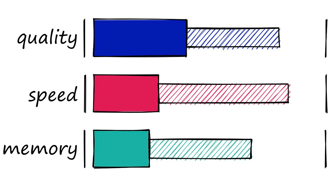
What we must do is identify where our use-case sweet spot lies. With flat indexes, we are here:

Here we have completely unoptimized search-speeds, which will fit many smaller index use-cases — or scenarios where search-time is irrelevant. But, other use-cases require a better balance speed and quality.
So, how can we make our search faster? There are two primary approaches:
- Reduce vector size — through dimensionality reduction or reducing the number of bits representing our vectors values.
- Reduce search scope — we can do this by clustering or organizing vectors into tree structures based on certain attributes, similarity, or distance — and restricting our search to closest clusters or filter through most similar branches.
Using either of these approaches means that we are no longer performing an exhaustive nearest-neighbors search but an approximate nearest-neighbors (ANN) search — as we no longer search the entire, full-resolution dataset.
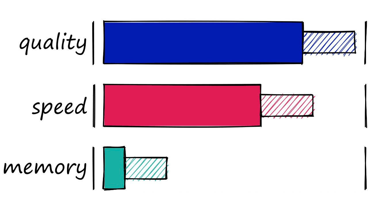
So, what we produce is a more balanced mix that prioritizes both search-speed and search-time:

Locality Sensitive Hashing
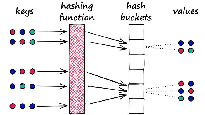
Locality Sensitive Hashing (LSH) works by grouping vectors into buckets by processing each vector through a hash function that maximizes hashing collisions — rather than minimizing as is usual with hashing functions.
What does that mean? Imagine we have a Python dictionary. When we create a new key-value pair in our dictionary, we use a hashing function to hash the key. This hash value of the key determines the ‘bucket’ where we store its respective value:
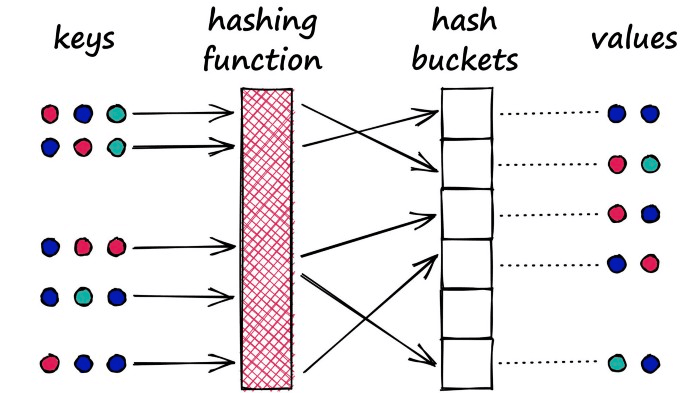
A Python dictionary is an example of a hash table using a typical hashing function that minimizes hashing collisions, a hashing collision where two different objects (keys) produce the same hash.
In our dictionary, we want to avoid these collisions as it means that we would have multiple objects mapped to a single key — but for LSH, we want to maximize hashing collisions.
Why would we want to maximize collisions? Well, for search, we use LSH to group similar objects together. When we introduce a new query object (or vector), our LSH algorithm can be used to find the closest matching groups:
Implementing LSH
Implementing our LSH index in Faiss is easy. We initialize a IndexLSH object, using the vector dimensions d and the nbits argument — and add our vectors like so:
nbits = d*4  # resolution of bucketed vectors
# initialize index and add vectors
index = faiss.IndexLSH(d, nbits)
index.add(wb)
# and search
D, I = index.search(xq, k)
Our nbits argument refers to the ‘resolution’ of the hashed vectors. A higher value means greater accuracy at the cost of more memory and slower search speeds.
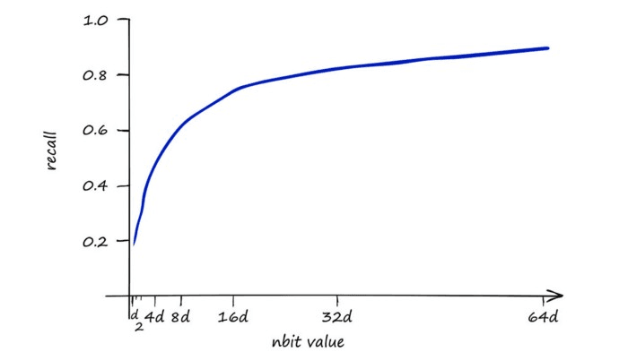
Our baseline IndexFlatIP index is our 100% recall performance, using IndexLSH we can achieve 90% using a very high nbits value.
This is a strong result — 90% of the performance could certainly be a reasonable sacrifice to performance if we get improved search-times.
However, LSH is highly sensitive to the curse of dimensionality when using a larger d value we also need to increase nbits to maintain search-quality.
So our stored vectors become increasingly larger as our original vector dimensionality d increases. This quickly leads to excessive search times:
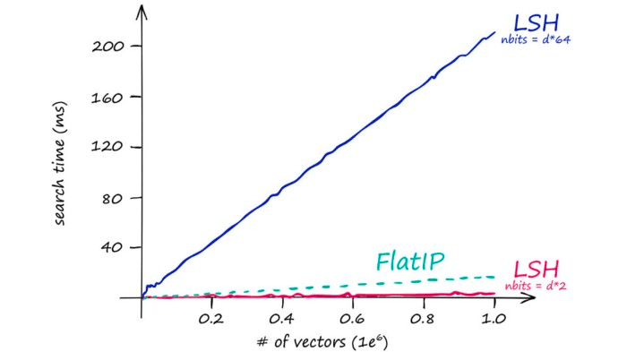
Which is mirrored by our index memory size:
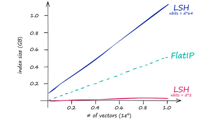
So IndexLSH is not suitable if we have large vector dimensionality (128 is already too large). Instead, it is best suited to low-dimensionality vectors — and small indexes.
If we find ourselves with large d values or large indexes — we avoid LSH completely, instead focusing on our next index, HNSW.
Hierarchical Navigable Small World Graphs
Hierarchical Navigable Small World (HNSW) graphs are another, more recent development in search. HNSW-based ANNS consistently top out as the highest performing indexes [1].
HNSW is a further adaption of navigable small world (NSW) graphs — where an NSW graph is a graph structure containing vertices connected by edges to their nearest neighbors.
The ‘NSW’ part is due to vertices within these graphs all having a very short average path length to all other vertices within the graph — despite not being directly connected.
Using the example of Facebook — in 2016, we could connect every user (a vertex) to their Facebook friends (their nearest neighbors). And despite the 1.59B active users, the average number of steps (or hops) needed to traverse the graph from one user to another was just 3.57 [2].
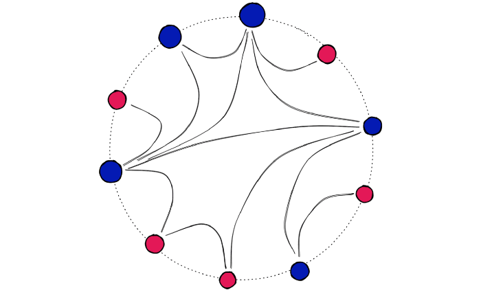
Facebook is just one example of high connectivity in vast networks — otherwise known as an NSW graph.
At a high level, HNSW graphs are built by taking NSW graphs and breaking them apart into multiple layers. With each incremental layer eliminating intermediate connections between vertices.
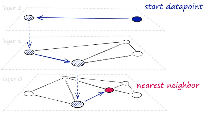
For bigger datasets with higher-dimensionality — HNSW graphs are some of the best performing indexes we can use. We’ll be covering using the HNSW index alone, but by layering other quantization steps, we can improve search-times even further.
HNSW Implementation
To build and search a flat HNSW index in Faiss, all we need is IndexHNSWFlat:
# set HNSW index parameters
M = 64  # number of connections each vertex will have
ef_search = 32  # depth of layers explored during search
ef_construction = 64  # depth of layers explored during index construction

# initialize index (d == 128)
index = faiss.IndexHNSWFlat(d, M)
# set efConstruction and efSearch parameters
index.hnsw.efConstruction = ef_construction
index.hnsw.efSearch = ef_search
# add data to index
index.add(wb)

# search as usual
D, I = index.search(wb, k)
Here, we have three key parameters for modifying our index performance.
M— the number of nearest neighbors that each vertex will connect to.efSearch— how many entry points will be explored between layers during the search.efConstruction— how many entry points will be explored when building the index.
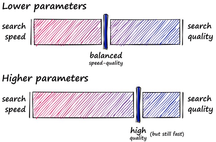
Each of these parameters can be increased to improve search-quality:
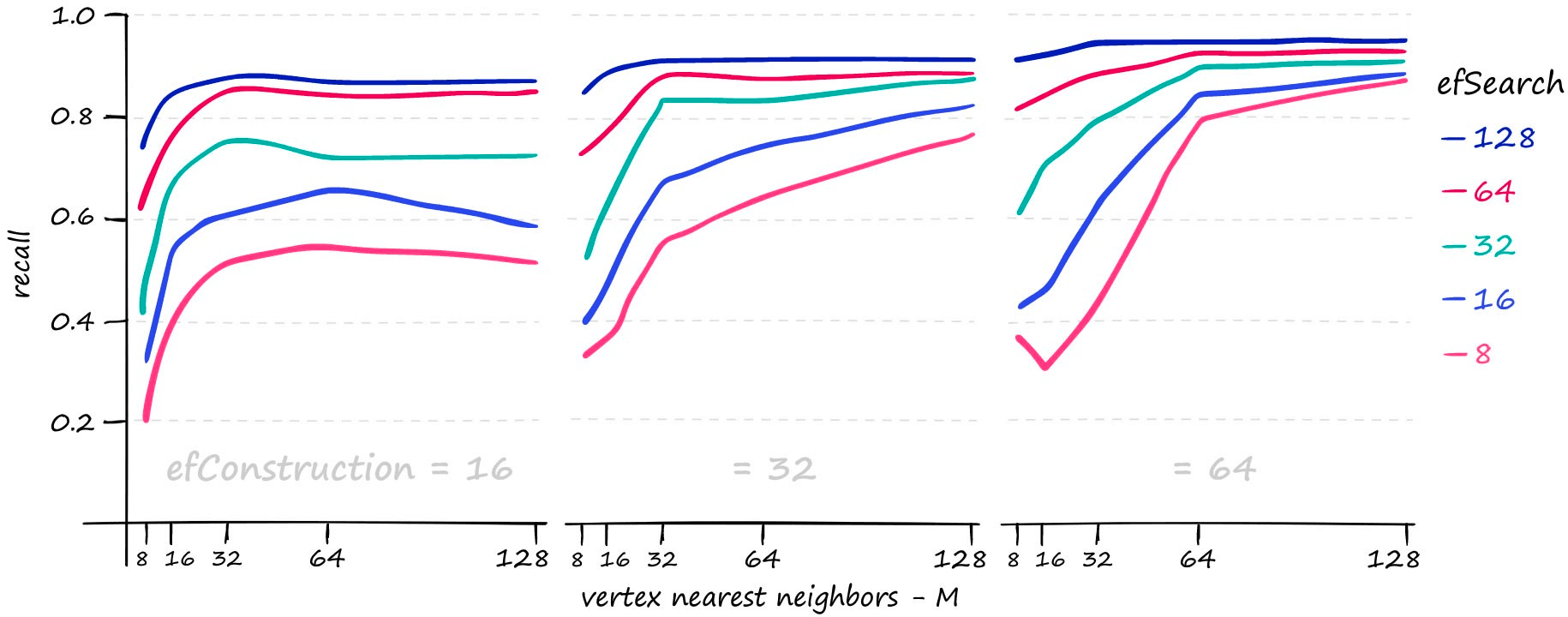
M and efSearch have a larger impact on search-time — efConstruction primarily increases index construction time (meaning a slower index.add), but at higher M values and higher query volume we do see an impact from efConstruction on search-time too.
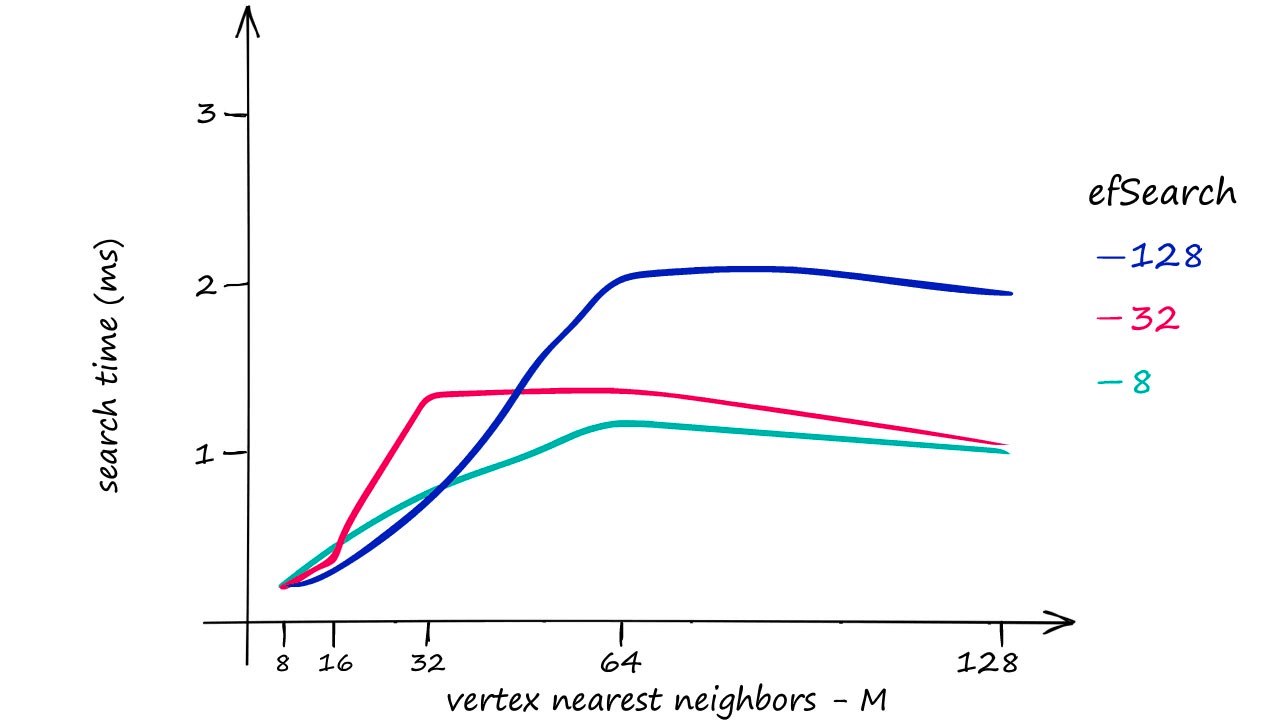
HNSW gives us great search-quality at very fast search-speeds — but there’s always a catch — HNSW indexes take up a significant amount of memory. Using an M value of 128 for the Sift1M dataset requires upwards of 1.6GB of memory.
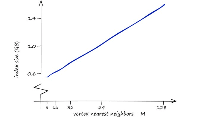
However, we can increase our other two parameters — efSearch and efConstruction with no effect on the index memory footprint.
So, where RAM is not a limiting factor HNSW is great as a well-balanced index that we can push to focus more towards quality by increasing our three parameters.
That’s HNSW in Faiss — an incredibly powerful and efficient index. Now let’s move onto our final index — IVF.
Inverted File Index
The Inverted File Index (IVF) index consists of search scope reduction through clustering. It’s a very popular index as it’s easy to use, with high search-quality and reasonable search-speed.
It works on the concept of Voronoi diagrams — also called Dirichlet tessellation (a much cooler name).
To understand Voronoi diagrams, we need to imagine our highly-dimensional vectors placed into a 2D space. We then place a few additional points in our 2D space, which will become our ‘cluster’ (Voronoi cells in our case) centroids.
We then extend an equal radius out from each of our centroids. At some point, the circumferences of each cell circle will collide with another — creating our cell edges:
Now, every datapoint will be contained within a cell — and be assigned to that respective centroid.
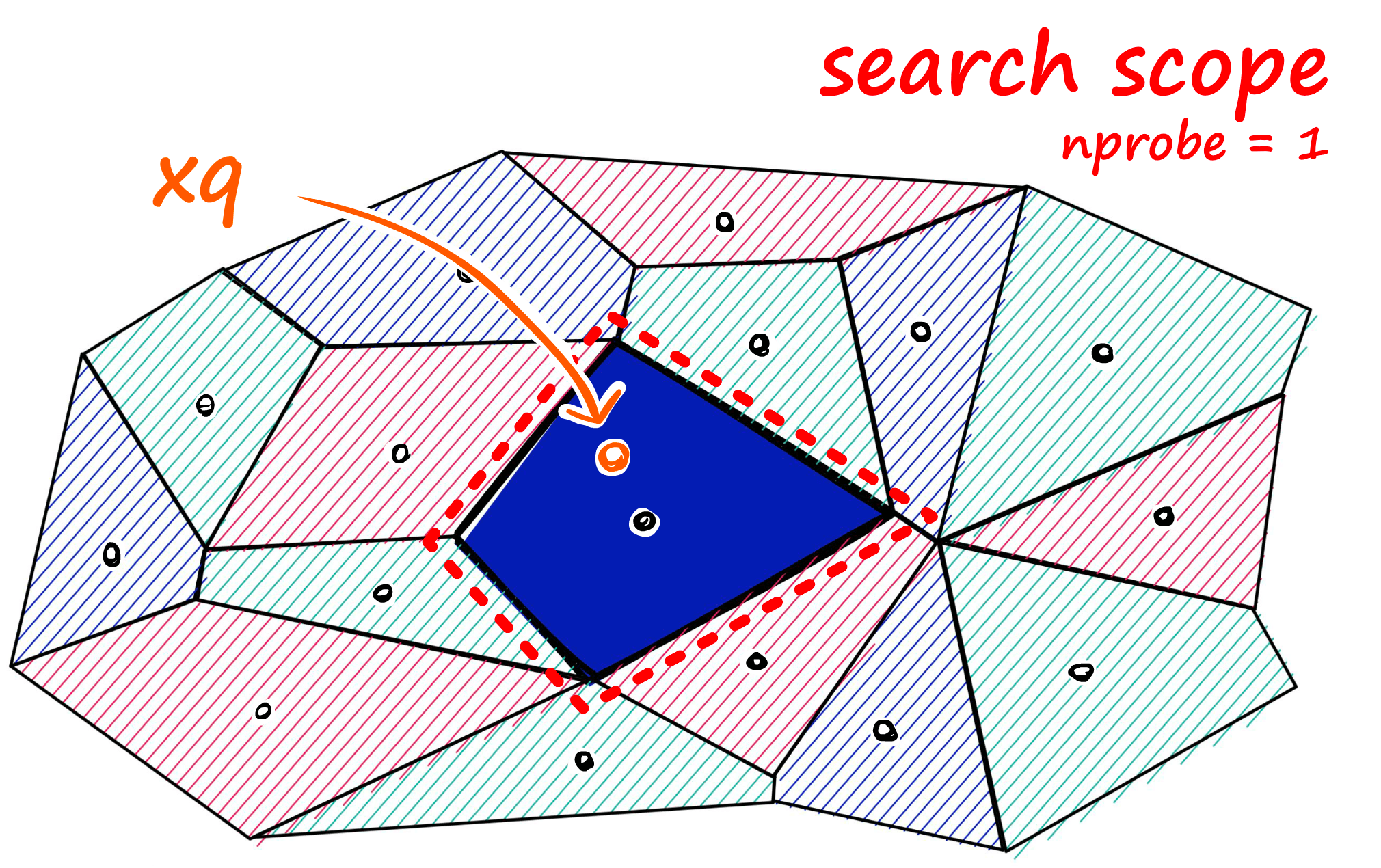
Just as with our other indexes, we introduce a query vector xq — this query vector must land within one of our cells, at which point we restrict our search scope to that single cell.
But there is a problem if our query vector lands near the edge of a cell — there’s a good chance that its closest other datapoint is contained within a neighboring cell. We call this the edge problem:
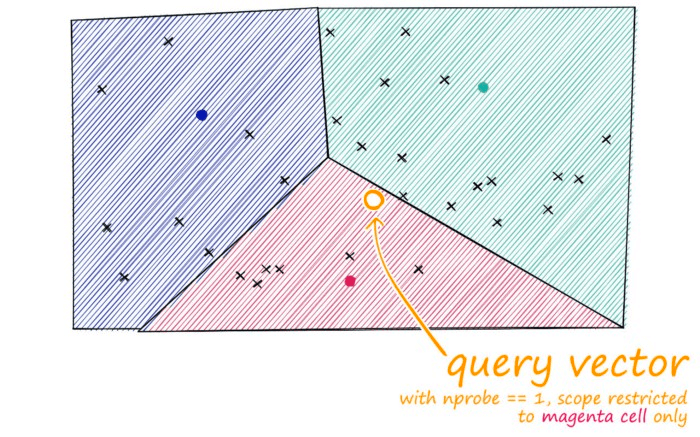
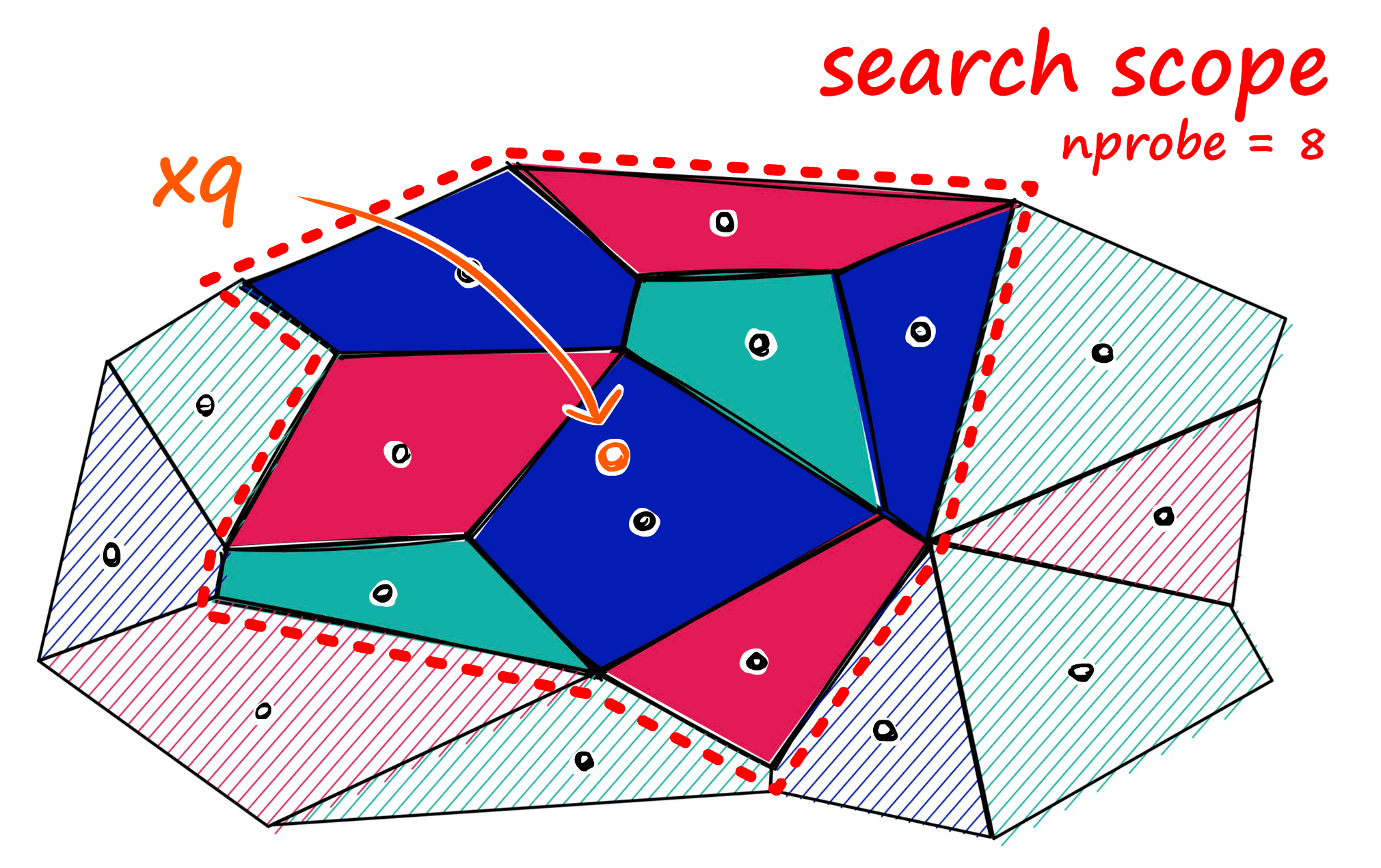
Now, what we can do to mitigate this issue and increase search-quality is increase an index parameter known as the nprobe value. With nprobe we can set the number of cells to search.
IVF Implementation
To implement an IVF index and use it in search, we can use IndexIVFFlat:
nlist = 128  # number of cells/clusters to partition data into

quantizer = faiss.IndexFlatIP(d)  # how the vectors will be stored/compared
index = faiss.IndexIVFFlat(quantizer, d, nlist)
index.train(data)  # we must train the index to cluster into cells
index.add(data)

index.nprobe = 8  # set how many of nearest cells to search
D, I = index.search(xq, k)
There are two parameters here that we can adjust.
nprobe— the number of cells to searchnlist— the number of cells to create
A higher nlist means that we must compare our vector to more centroid vectors — but after selecting the nearest centroid’s cells to search, there will be fewer vectors within each cell. So, increase nlist to prioritize search-speed.
As for nprobe, we find the opposite. Increasing nprobe increases the search scope — thus prioritizing search-quality.
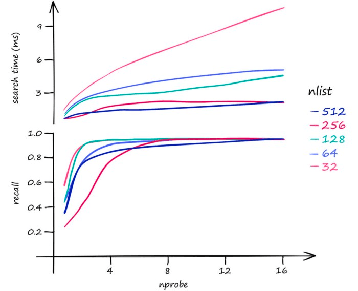
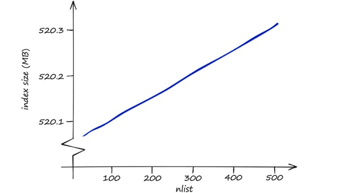
In terms of memory, IndexIVFFlat is reasonably efficient — and modifying nprobe will not affect this. The effect of nlist on memory usage is small too — higher nlist means a marginally larger memory requirement.
So, we must decide between greater search-quality with nprobe and faster search-speed with nlist.
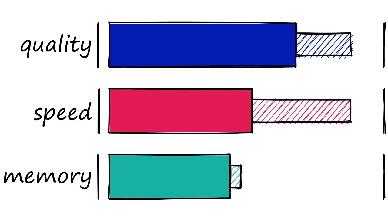
We’ve covered a lot in this article , so let’s wrap everything up with a quick summary of each index’s memory, speed, and search-quality performance.
| Index | Memory (MB) | Query Time (ms) | Recall | Notes |
|---|---|---|---|---|
| Flat (L2 or IP) | ~500 | ~18 | 1.0 | Good for small datasets or where query time is irrelevant |
| LSH | 20 - 600 | 1.7 - 30 | 0.4 - 0.85 | Best for low dimensional data, or small datasets |
| HNSW | 600 - 1600 | 0.6 - 2.1 | 0.5 - 0.95 | Very good for quality, high speed, but large memory usage |
| IVF | ~520 | 1 - 9 | 0.7 - 0.95 | Good scalable option. High-quality, at reasonable speed and memory usage |
Values displayed here are the range of values experienced during testing of each index on the Sift1M dataset and represent the average results from 20 tests at each parameter setting. Unrealistic parameter settings tested in this article (excessively low/high) have been excluded from this range.
The Sift1M dataset consists of a dimensionality d of 128, dataset size of 1M. The above values result from querying for a single vector - returning k == 10 of the nearest matches.
Hardware used
- M1 chip with 8-core CPU
- 8GB unified memory
So we have four indexes, with equally potent pros and cons — depending on the use-case. Hopefully, with this article, you will now be much better prepared to decide which of these indexes best fits your own use case.
Beyond these metrics, it is possible to improve memory usage and search-speed even further by adding other quantization or compression steps — but that is for another article.
References
[1] E Bernhardsson, ANN-benchmarks repo, Github
[2] S Edunov, et al., Three and a half degrees of separation (2016), Facebook Research
All images are by the author except where stated otherwise
Was this article helpful?