Sentence Transformers: Meanings in Disguise
Once you learn about and generate sentence embeddings, combine them with the Pinecone vector database to easily build applications like semantic search, deduplication, and multi-modal search. Try it now for free.
Transformers have wholly rebuilt the landscape of natural language processing (NLP). Before transformers, we had okay translation and language classification thanks to recurrent neural nets (RNNs) — their language comprehension was limited and led to many minor mistakes, and coherence over larger chunks of text was practically impossible.
Since the introduction of the first transformer model in the 2017 paper ‘Attention is all you need’ [1], NLP has moved from RNNs to models like BERT and GPT. These new models can answer questions, write articles (maybe GPT-3 wrote this), enable incredibly intuitive semantic search — and much more.
The funny thing is, for many tasks, the latter parts of these models are the same as those in RNNs — often a couple of feedforward NNs that output model predictions.
It’s the input to these layers that changed. The dense embeddings created by transformer models are so much richer in information that we get massive performance benefits despite using the same final outward layers.
These increasingly rich sentence embeddings can be used to quickly compare sentence similarity for various use cases. Such as:
- Semantic textual similarity (STS) — comparison of sentence pairs. We may want to identify patterns in datasets, but this is most often used for benchmarking.
- Semantic search — information retrieval (IR) using semantic meaning. Given a set of sentences, we can search using a ‘query’ sentence and identify the most similar records. Enables search to be performed on concepts (rather than specific words).
- Clustering — we can cluster our sentences, useful for topic modeling.
In this article, we will explore how these embeddings have been adapted and applied to a range of semantic similarity applications by using a new breed of transformers called ‘sentence transformers’.
Some “Context”
Before we dive into sentence transformers, it might help to piece together why transformer embeddings are so much richer — and where the difference lies between a vanilla transformer and a sentence transformer.
Transformers are indirect descendants of the previous RNN models. These old recurrent models were typically built from many recurrent units like LSTMs or GRUs.
In machine translation, we would find encoder-decoder networks. The first model for encoding the original language to a context vector, and a second model for decoding this into the target language.
Encoder-decoder architecture with the single context vector shared between the two models, this acts as an information bottleneck as all information must be passed through this point.
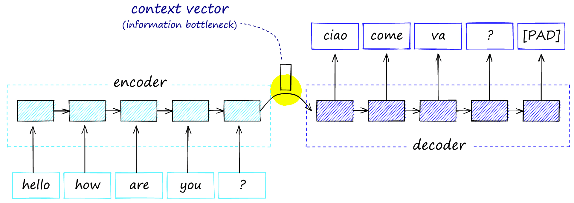
The problem here is that we create an information bottleneck between the two models. We’re creating a massive amount of information over multiple time steps and trying to squeeze it all through a single connection. This limits the encoder-decoder performance because much of the information produced by the encoder is lost before reaching the decoder.
The attention mechanism provided a solution to the bottleneck issue. It offered another route for information to pass through. Still, it didn’t overwhelm the process because it focused attention only on the most relevant information.
By passing a context vector from each timestep into the attention mechanism (producing annotation vectors), the information bottleneck is removed, and there is better information retention across longer sequences.
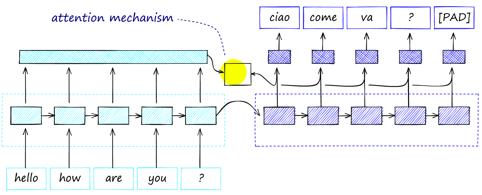
During decoding, the model decodes one word/timestep at a time. An alignment (e.g., similarity) between the word and all encoder annotations is calculated for each step.
Higher alignment resulted in greater weighting to the encoder annotation on the output of the decoder step. Meaning the mechanism calculated which encoder words to pay attention to.
![Attention between an English-French encoder and decoder, source [2].](/_next/image/?url=https%3A%2F%2Fcdn.sanity.io%2Fimages%2Fvr8gru94%2Fproduction%2Fab5024ccb25d38298b19f6da73eed1f5b1f9579e-1400x871.png&w=3840&q=75)
The best-performing RNN encoder-decoders all used this attention mechanism.
Attention is All You Need
In 2017, a paper titled Attention Is All You Need was published. This marked a turning point in NLP. The authors demonstrated that we could remove the RNN networks and get superior performance using just the attention mechanism — with a few changes.
This new attention-based model was named a ‘transformer’. Since then, the NLP ecosystem has entirely shifted from RNNs to transformers thanks to their vastly superior performance and incredible capability for generalization.
The first transformer removed the need for RNNs through the use of three key components:
- Positional Encoding
- Self-attention
- Multi-head attention
Positional encoding replaced the key advantage of RNNs in NLP — the ability to consider the order of a sequence (they were recurrent). It worked by adding a set of varying sine wave activations to each input embedding based on position.
Self-attention is where the attention mechanism is applied between a word and all of the other words in its own context (sentence/paragraph). This is different from vanilla attention which specifically focused on attention between encoders and decoders.
Multi-head attention can be seen as several parallel attention mechanisms working together. Using several attention heads allowed the representation of several sets of relationships (rather than a single set).
Pretrained Models
The new transformer models generalized much better than previous RNNs, which were often built specifically for each use-case.
With transformer models, it is possible to use the same ‘core’ of a model and simply swap the last few layers for different use cases (without retraining the core).
This new property resulted in the rise of pretrained models for NLP. Pretrained transformer models are trained on vast amounts of training data — often at high costs by the likes of Google or OpenAI, then released for the public to use for free.
One of the most widely used of these pretrained models is BERT, or Bidirectional Encoder Representations from Transformers by Google AI.
BERT spawned a whole host of further models and derivations such as distilBERT, RoBERTa, and ALBERT, covering tasks such as classification, Q&A, POS-tagging, and more.
BERT for Sentence Similarity
So far, so good, but these transformer models had one issue when building sentence vectors: Transformers work using word or token-level embeddings, not sentence-level embeddings.
Before sentence transformers, the approach to calculating accurate sentence similarity with BERT was to use a cross-encoder structure. This meant that we would pass two sentences to BERT, add a classification head to the top of BERT — and use this to output a similarity score.
The BERT cross-encoder architecture consists of a BERT model which consumes sentences A and B. Both are processed in the same sequence, separated by a [SEP] token. All of this is followed by a feedforward NN classifier that outputs a similarity score.
![The BERT cross-encoder architecture consists of a BERT model which consumes sentences A and B. Both are processed in the same sequence, separated by a [SEP] token. All of this is followed by a feedforward NN classifier that outputs a similarity score.](/_next/image/?url=https%3A%2F%2Fcdn.sanity.io%2Fimages%2Fvr8gru94%2Fproduction%2F9a89f1b7dddd4c78da8b9ba0311c2ffd1ff18ffe-1920x1080.png&w=3840&q=75)
The cross-encoder network does produce very accurate similarity scores (better than SBERT), but it’s not scalable. If we wanted to perform a similarity search through a small 100K sentence dataset, we would need to complete the cross-encoder inference computation 100K times.
To cluster sentences, we would need to compare all sentences in our 100K dataset, resulting in just under 500M comparisons — this is simply not realistic.
Ideally, we need to pre-compute sentence vectors that can be stored and then used whenever required. If these vector representations are good, all we need to do is calculate the cosine similarity between each.
With the original BERT (and other transformers), we can build a sentence embedding by averaging the values across all token embeddings output by BERT (if we input 512 tokens, we output 512 embeddings). Alternatively, we can use the output of the first [CLS] token (a BERT-specific token whose output embedding is used in classification tasks).
Using one of these two approaches gives us our sentence embeddings that can be stored and compared much faster, shifting search times from 65 hours to around 5 seconds (see below). However, the accuracy is not good, and is worse than using averaged GloVe embeddings (which were developed in 2014).
The solution to this lack of an accurate model with reasonable latency was designed by Nils Reimers and Iryna Gurevych in 2019 with the introduction of sentence-BERT (SBERT) and the sentence-transformers library.
SBERT outperformed the previous state-of-the-art (SOTA) models for all common semantic textual similarity (STS) tasks — more on these later — except a single dataset (SICK-R).
Thankfully for scalability, SBERT produces sentence embeddings — so we do not need to perform a whole inference computation for every sentence-pair comparison.
Reimers and Gurevych demonstrated the dramatic speed increase in 2019. Finding the most similar sentence pair from 10K sentences took 65 hours with BERT. With SBERT, embeddings are created in ~5 seconds and compared with cosine similarity in ~0.01 seconds.
Since the SBERT paper, many more sentence transformer models have been built using similar concepts that went into training the original SBERT. They’re all trained on many similar and dissimilar sentence pairs.
Using a loss function such as softmax loss, multiple negatives ranking loss, or MSE margin loss, these models are optimized to produce similar embeddings for similar sentences, and dissimilar embeddings otherwise.
Now you have some context behind sentence transformers, where they come from, and why they’re needed. Let’s dive into how they work.
[3] The SBERT paper covers many of the statements, techniques, and numbers from this section.
Sentence Transformers
We explained the cross-encoder architecture for sentence similarity with BERT. SBERT is similar but drops the final classification head, and processes one sentence at a time. SBERT then uses mean pooling on the final output layer to produce a sentence embedding.
Unlike BERT, SBERT is fine-tuned on sentence pairs using a siamese architecture. We can think of this as having two identical BERTs in parallel that share the exact same network weights.
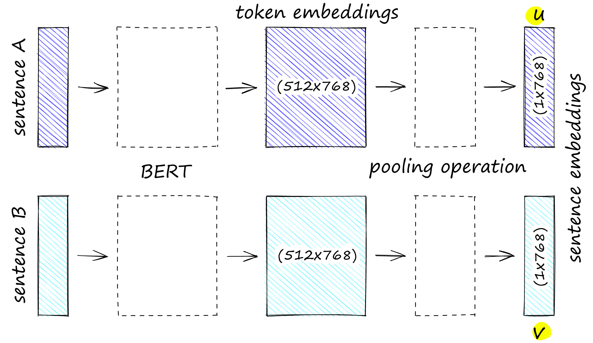
In reality, we are using a single BERT model. However, because we process sentence A followed by sentence B as pairs during training, it is easier to think of this as two models with tied weights.
Siamese BERT Pre-Training
There are different approaches to training sentence transformers. We will describe the original process featured most prominently in the original SBERT that optimizes on softmax-loss. Note that this is a high-level explanation, we will save the in-depth walkthrough for another article.
The softmax-loss approach used the ‘siamese’ architecture fine-tuned on the Stanford Natural Language Inference (SNLI) and Multi-Genre NLI (MNLI) corpora.
SNLI contains 570K sentence pairs, and MNLI contains 430K. The pairs in both corpora include a premise and a hypothesis. Each pair is assigned one of three labels:
- 0 — entailment, e.g. the
premisesuggests thehypothesis. - 1 — neutral, the
premiseandhypothesiscould both be true, but they are not necessarily related. - 2 — contradiction, the
premiseandhypothesiscontradict each other.
Given this data, we feed sentence A (let’s say the premise) into siamese BERT A and sentence B (hypothesis) into siamese BERT B.
The siamese BERT outputs our pooled sentence embeddings. There were the results of three different pooling methods in the SBERT paper. Those are mean, max, and [CLS]-pooling. The mean-pooling approach was best performing for both NLI and STSb datasets.
There are now two sentence embeddings. We will call embeddings A u and embeddings B v. The next step is to concatenate u and v. Again, several concatenation approaches were tested, but the highest performing was a (u, v, |u-v|) operation:
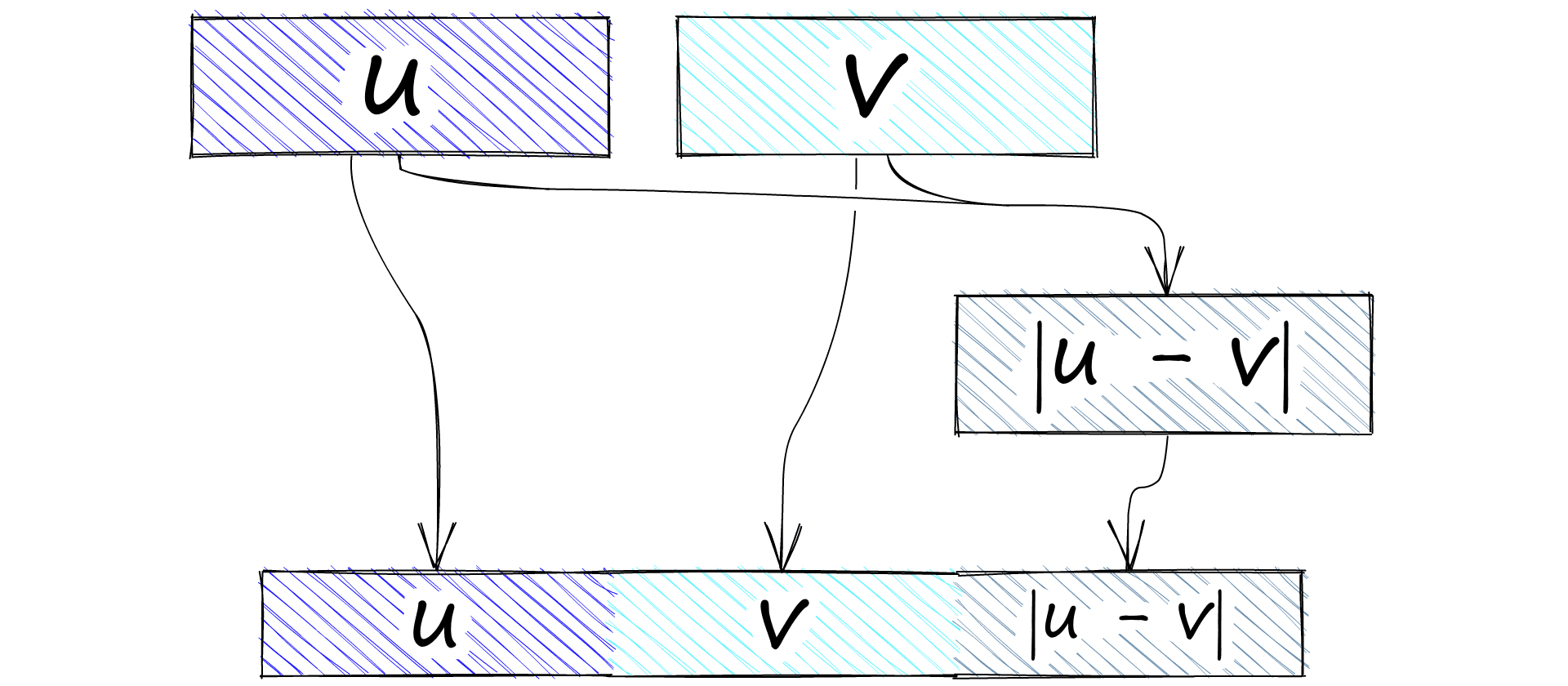
|u-v| is calculated to give us the element-wise difference between the two vectors. Alongside the original two embeddings (u and v), these are all fed into a feedforward neural net (FFNN) that has three outputs.
These three outputs align to our NLI similarity labels 0, 1, and 2. We need to calculate the softmax from our FFNN, which is done within the cross-entropy loss function. The softmax and labels are used to optimize on this ‘softmax-loss’.
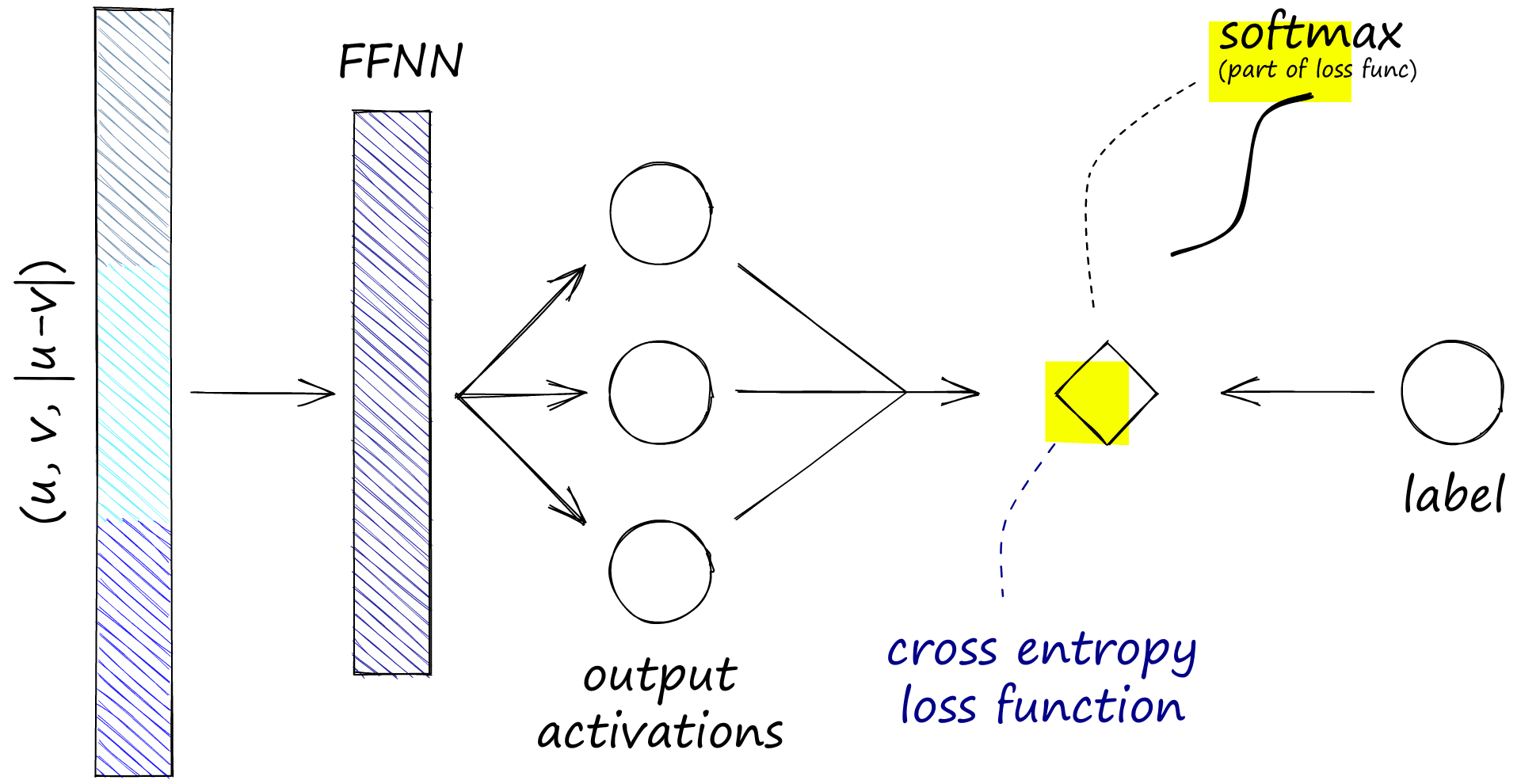
The operations were performed during training on two sentence embeddings, u and v. Note that softmax-loss refers cross-entropy loss (which contains a softmax function by default).
This results in our pooled sentence embeddings for similar sentences (label 0) becoming more similar, and embeddings for dissimilar sentences (label 2) becoming less similar.
Remember we are using siamese BERTs not dual BERTs. Meaning we don’t use two independent BERT models but a single BERT that processes sentence A followed by sentence B.
This means that when we optimize the model weights, they are pushed in a direction that allows the model to output more similar vectors where we see an entailment label and more dissimilar vectors where we see a contradiction label.
We are working on a step-by-step guide to training a siamese BERT model with the SNLI and MNLI corpora described above using both the softmax-loss and multiple-negatives-ranking-loss approaches. You can get an email as soon as we release the article by clicking here (the form is at the bottom of the page).
The fact that this training approach works is not particularly intuitive and indeed has been described by Reimers as coincidentally producing good sentence embeddings [5].
Since the original paper, further work has been done in this area. Many more models such as the latest MPNet and RoBERTa models trained on 1B+ samples (producing much better performance) have been built. We will be exploring some of these in future articles, and the superior training approaches they use.
For now, let’s look at how we can initialize and use some of these sentence-transformer models.
Getting Started with Sentence Transformers
The fastest and easiest way to begin working with sentence transformers is through the sentence-transformers library created by the creators of SBERT. We can install it with pip.
!pip install sentence-transformersWe will start with the original SBERT model bert-base-nli-mean-tokens. First, we download and initialize the model.
from sentence_transformers import SentenceTransformer

model = SentenceTransformer('bert-base-nli-mean-tokens')

modelSentenceTransformer(
(0): Transformer({'max_seq_length': 128, 'do_lower_case': False}) with Transformer model: BertModel
(1): Pooling({'word_embedding_dimension': 768, 'pooling_mode_cls_token': False, 'pooling_mode_mean_tokens': True, 'pooling_mode_max_tokens': False, 'pooling_mode_mean_sqrt_len_tokens': False})
)The output we can see here is the SentenceTransformer object which contains three components:
- The transformer itself, here we can see the max sequence length of
128tokens and whether to lowercase any input (in this case, the model does not). We can also see the model class,BertModel. - The pooling operation, here we can see that we are producing a
768-dimensional sentence embedding. We are doing this using the mean pooling method.
Once we have the model, building sentence embeddings is quickly done using the encode method.
sentences = [
    "the fifty mannequin heads floating in the pool kind of freaked them out",
    "she swore she just saw her sushi move",
    "he embraced his new life as an eggplant",
    "my dentist tells me that chewing bricks is very bad for your teeth",
    "the dental specialist recommended an immediate stop to flossing with construction materials"
]

embeddings = model.encode(sentences)

embeddings.shape(5, 768)We now have sentence embeddings that we can use to quickly compare sentence similarity for the use cases introduced at the start of the article; STS, semantic search, and clustering.
We can put together a fast STS example using nothing more than a cosine similarity function and Numpy.
import numpy as np
from sentence_transformers.util import cos_sim

sim = np.zeros((len(sentences), len(sentences)))

for i in range(len(sentences)):
    sim[i:,i] = cos_sim(embeddings[i], embeddings[i:])

simarray([[1.00000024, 0. , 0. , 0. , 0. ],
[0.40914285, 1. , 0. , 0. , 0. ],
[0.10909 , 0.4454796 , 1. , 0. , 0. ],
[0.50074852, 0.30693918, 0.20791623, 0.99999958, 0. ],
[0.29936209, 0.38607228, 0.28499269, 0.63849503, 1.0000006 ]])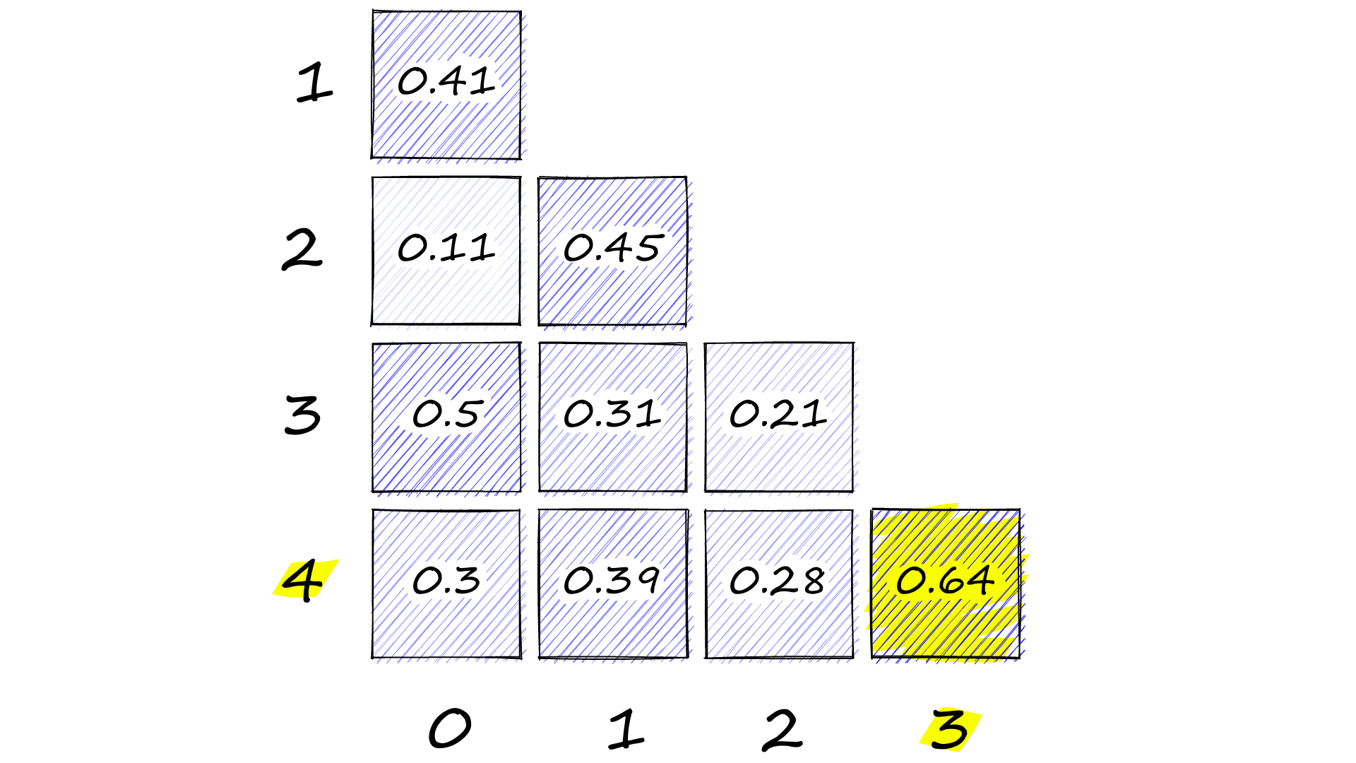
Here we have calculated the cosine similarity between every combination of our five sentence embeddings. Which are:
| Index | Sentence |
|---|---|
| 0 | the fifty mannequin heads floating in the pool kind of freaked them out |
| 1 | she swore she just saw her sushi move |
| 2 | he embraced his new life as an eggplant |
| 3 | my dentist tells me that chewing bricks is very bad for your teeth |
| 4 | the dental specialist recommended an immediate stop to flossing with construction materials |
IndexSentence0the fifty mannequin heads floating in the pool kind of freaked them out1she swore she just saw her sushi move2he embraced his new life as an eggplant3my dentist tells me that chewing bricks is very bad for your teeth4the dental specialist recommended an immediate stop to flossing with construction materials
We can see the highest similarity score in the bottom-right corner with 0.64. As we would hope, this is for sentences 4 and 3, which both describe poor dental practices using construction materials.
Other sentence-transformers
Although we returned good results from the SBERT model, many more sentence transformer models have since been built. Many of which we can find in the sentence-transformers library.
These newer models can significantly outperform the original SBERT. In fact, SBERT is no longer listed as an available model on the SBERT.net models page.
| Model | Avg. Performance | Speed | Size (MB) |
|---|---|---|---|
| all-mpnet-base-v2 | 63.30 | 2800 | 418 |
| all-roberta-large-v1 | 53.05 | 800 | 1355 |
| all-MiniLM-L12-v1 | 59.80 | 7500 | 118 |
We will cover some of these later models in more detail in future articles. For now, let’s compare one of the highest performers and run through our STS task.
# !pip install sentence-transformers

from sentence_transformers import SentenceTransformer

mpnet = SentenceTransformer('all-mpnet-base-v2')

mpnetSentenceTransformer(
(0): Transformer({'max_seq_length': 384, 'do_lower_case': False}) with Transformer model: MPNetModel
(1): Pooling({'word_embedding_dimension': 768, 'pooling_mode_cls_token': False, 'pooling_mode_mean_tokens': True, 'pooling_mode_max_tokens': False, 'pooling_mode_mean_sqrt_len_tokens': False})
(2): Normalize()
)Here we have the SentenceTransformer model for all-mpnet-base-v2. The components are very similar to the bert-base-nli-mean-tokens model, with some small differences:
max_seq_lengthhas increased from128to384. Meaning we can process sequences that are three times longer than we could with SBERT.- The base model is now
MPNetModel[4] notBertModel. - There is an additional normalization layer applied to sentence embeddings.
Let’s compare the STS results of all-mpnet-base-v2 against SBERT.
embeddings = mpnet.encode(sentences)

sim = np.zeros((len(sentences), len(sentences)))

for i in range(len(sentences)):
    sim[i:,i] = cos_sim(embeddings[i], embeddings[i:])

simarray([[ 1.00000048, 0. , 0. , 0. , 0. ],
[ 0.26406282, 1.00000012, 0. , 0. , 0. ],
[ 0.16503485, 0.16126671, 1.00000036, 0. , 0. ],
[ 0.04334451, 0.04615867, 0.0567013 , 1.00000036, 0. ],
[ 0.05398509, 0.06101188, -0.01122264, 0.51847214, 0.99999952]])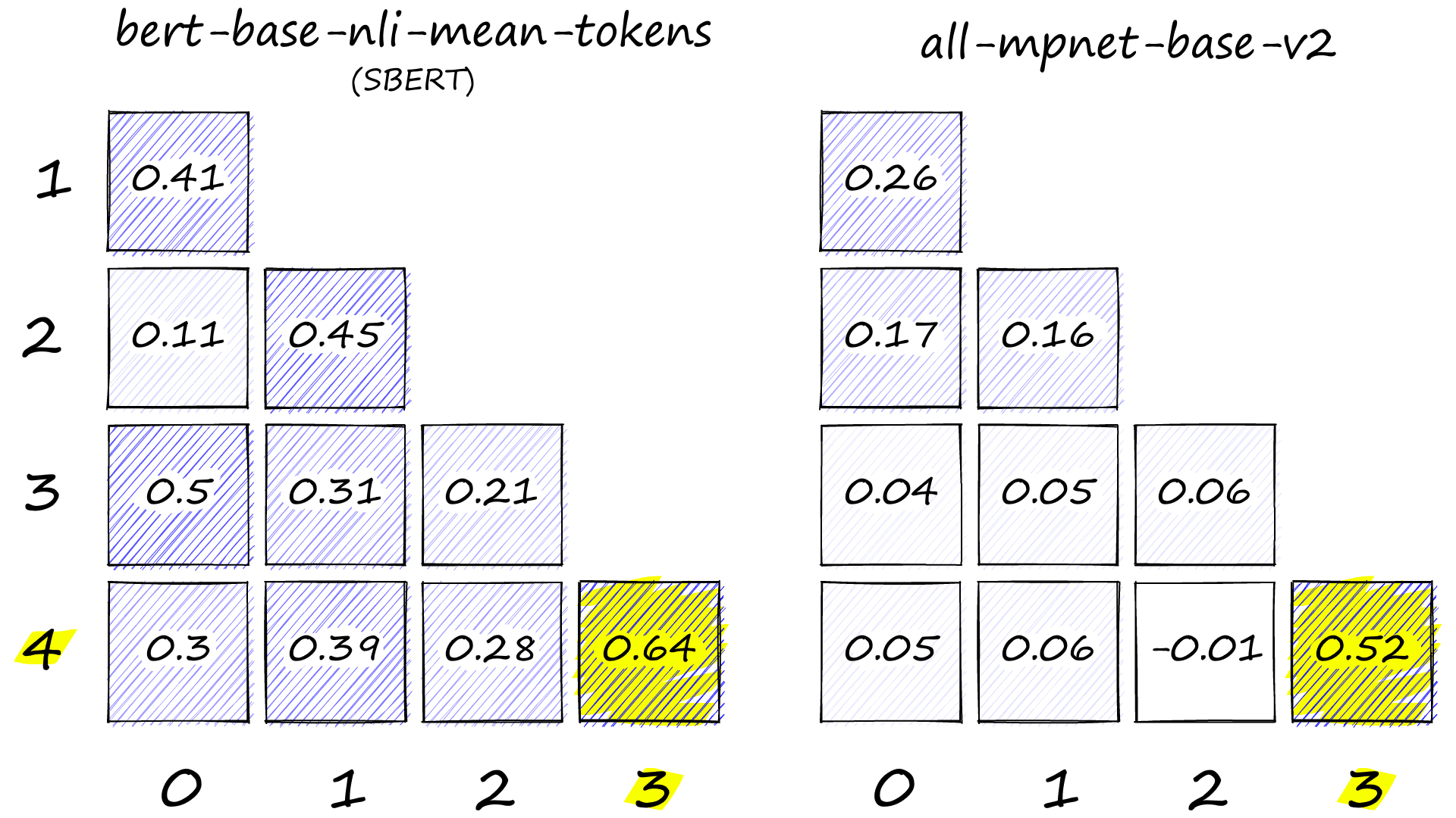
The semantic representation of later models is apparent. Although SBERT correctly identifies 4 and 3 as the most similar pair, it also assigns reasonably high similarity to other sentence pairs.
On the other hand, the MPNet model makes a very clear distinction between similar and dissimilar pairs, with most pairs scoring less than 0.1 and the 4-3 pair scored at 0.52.
By increasing the separation between dissimilar and similar pairs, we’re:
- Making it easier to automatically identify relevant pairs.
- Pushing predictions closer to the 0 and 1 target scores for dissimilar and similar pairs used during training. This is something we will see more of in our future articles on fine-tuning these models.
That’s it for this article introducing sentence embeddings and the current SOTA sentence transformer models for building these incredibly useful embeddings.
Sentence embeddings, although only recently popularized, were produced from a long range of fantastic innovations. We described some of the mechanics applied to create the first sentence transformer, SBERT.
We also demonstrated that despite SBERT’s very recent introduction in 2019, other sentence transformers already outperform the model. Fortunately for us, it’s easy to switch out SBERT for one of these newer models with the sentence-transformers library.
In future articles, we will dive deeper into some of these newer models and how to train our own sentence transformers.
Subscribe for more semantic search material!Submit
References
[1] A. Vashwani, et al., Attention Is All You Need (2017), NeurIPS
[2] D. Bahdanau, et al., Neural Machine Translation by Jointly Learning to Align and Translate (2015), ICLR
[3] N. Reimers, I. Gurevych, Sentence-BERT: Sentence Embeddings using Siamese BERT-Networks (2019), ACL
[4] MPNet Model, Hugging Face Docs
[5] N. Reimers, Natural Language Inference, sentence-transformers on GitHub
Was this article helpful?