Locality Sensitive Hashing (LSH): The Illustrated Guide
Locality sensitive hashing (LSH) is a widely popular technique used in approximate nearest neighbor (ANN) search. The solution to efficient similarity search is a profitable one — it is at the core of several billion (and even trillion) dollar companies.
Big names like Google, Netflix, Amazon, Spotify, Uber, and countless more rely on similarity search for many of their core functions.
Amazon uses similarity search to compare customers, finding new product recommendations based on the purchasing history of their highest-similarity customers.
Every time you use Google, you perform a similarity search between your query/search term — and Google’s indexed internet.
If Spotify manages to recommend good music, it’s because their similarity search algorithms are successfully matching you to other customers with a similarly good (or not so good) taste in music.
LSH is one of the original techniques for producing high quality search, while maintaining lightning fast search speeds. In this article we will work through the theory behind the algorithm, alongside an easy-to-understand implementation in Python!
You can find a video walkthrough of this article here:
Search Complexity
Imagine a dataset containing millions or even billions of samples — how can we efficiently compare all of those samples?
Even on the best hardware, comparing all pairs is out of the question. This produces an at best complexity of O(n²). Even if comparing a single query against the billions of samples, we still return an at best complexity of O(n).
We also need to consider the complexity behind a single similarity calculation — every sample is stored as a vector, often very highly-dimensional vectors — this increases our complexity even further.
How can we avoid this? Is it even possible to perform a search with sub-linear complexity? Yes, it is!
The solution is approximate search. Rather than comparing every vector (exhaustive search) — we can approximate and limit our search scope to only the most relevant vectors.
LSH is one algorithm that provides us with those sub-linear search times. In this article, we will introduce LSH and work through the logic behind the magic.
Locality Sensitive Hashing
When we consider the complexity of finding similar pairs of vectors, we find that the number of calculations required to compare everything is unmanageably enormous even with reasonably small datasets.
Let’s consider a vector index. If we were to introduce just one new vector and attempt to find the closest match — we must compare that vector to every other vector in our database. This gives us a linear time complexity — which cannot scale to fast search in larger datasets.
The problem is even worse if we wanted to compare all of those vectors against each other — the optimal approach sorting method to achieve this is at best log-linear time complexity.
So we need a way to reduce the number of comparisons. Ideally, we want only to compare vectors that we believe to be potential matches — or candidate pairs.
Locality sensitive hashing (LSH) allows us to do this.
LSH consists of a variety of different methods. In this article, we’ll be covering the traditional approach — which consists of multiple steps — shingling, MinHashing, and the final banded LSH function.
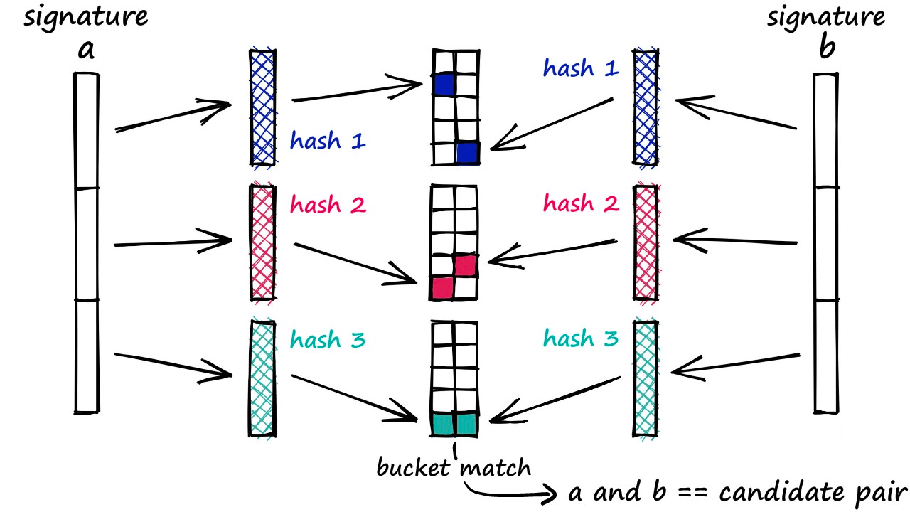
At its core, the final LSH function allows us to segment and hash the same sample several times. And when we find that a pair of vectors has been hashed to the same value at least once , we tag them as candidate pairs — that is, potential matches.
It is a very similar process to that used in Python dictionaries. We have a key-value pair which we feed into the dictionary. The key is processed through the dictionary hash function and mapped to a specific bucket. We then connect the respective value to this bucket.
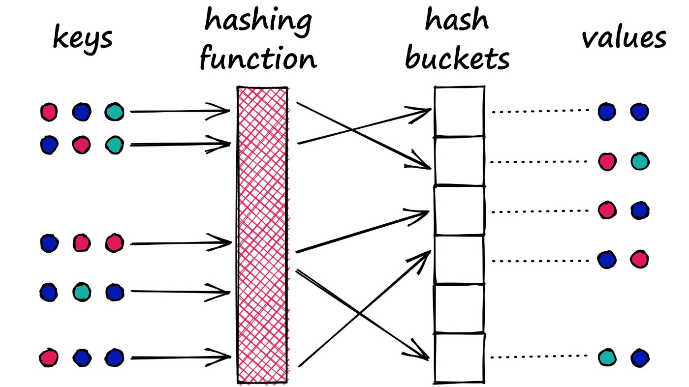
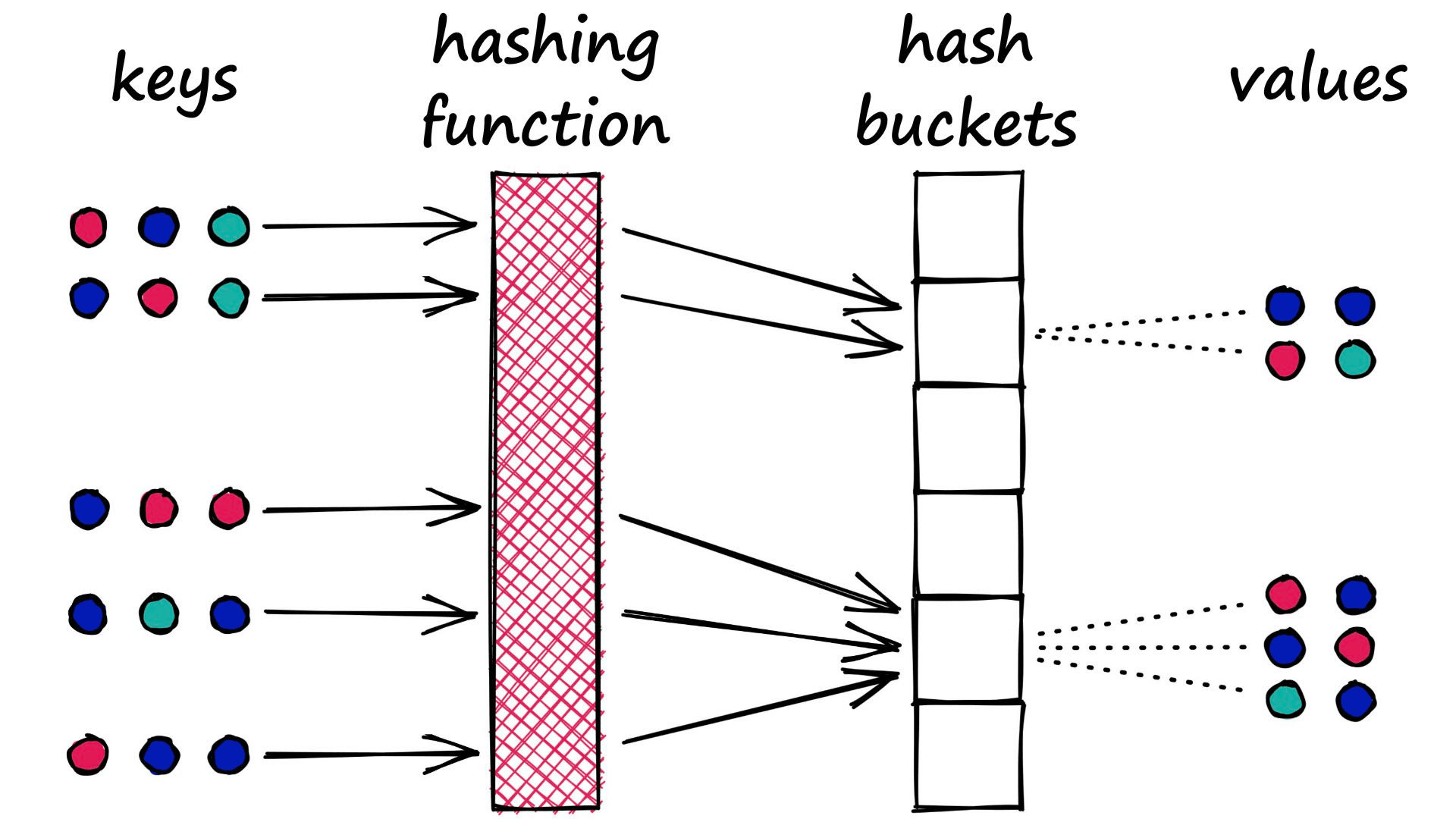
However, there is a key difference between this type of hash function and that used in LSH. With dictionaries, our goal is to minimize the chances of multiple key-values being mapped to the same bucket — we minimize collisions.
LSH is almost the opposite. In LSH, we want to maximize collisions — although ideally only for similar inputs.
There is no single approach to hashing in LSH. Indeed, they all share the same ‘bucket similar samples through a hash function’ logic , but they can vary a lot beyond this.
The method we have briefly described and will be covering throughout the remainder of this article could be described as the traditional approach, using shingling, MinHashing, and banding.
There are several other techniques, such as Random Projection which we cover in another article.
Shingling, MinHashing, and LSH
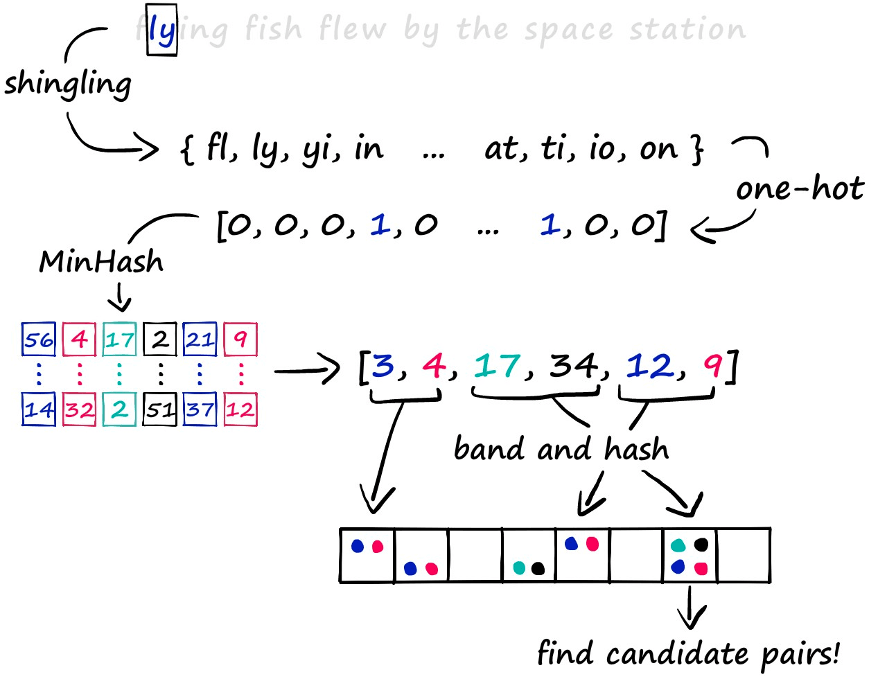
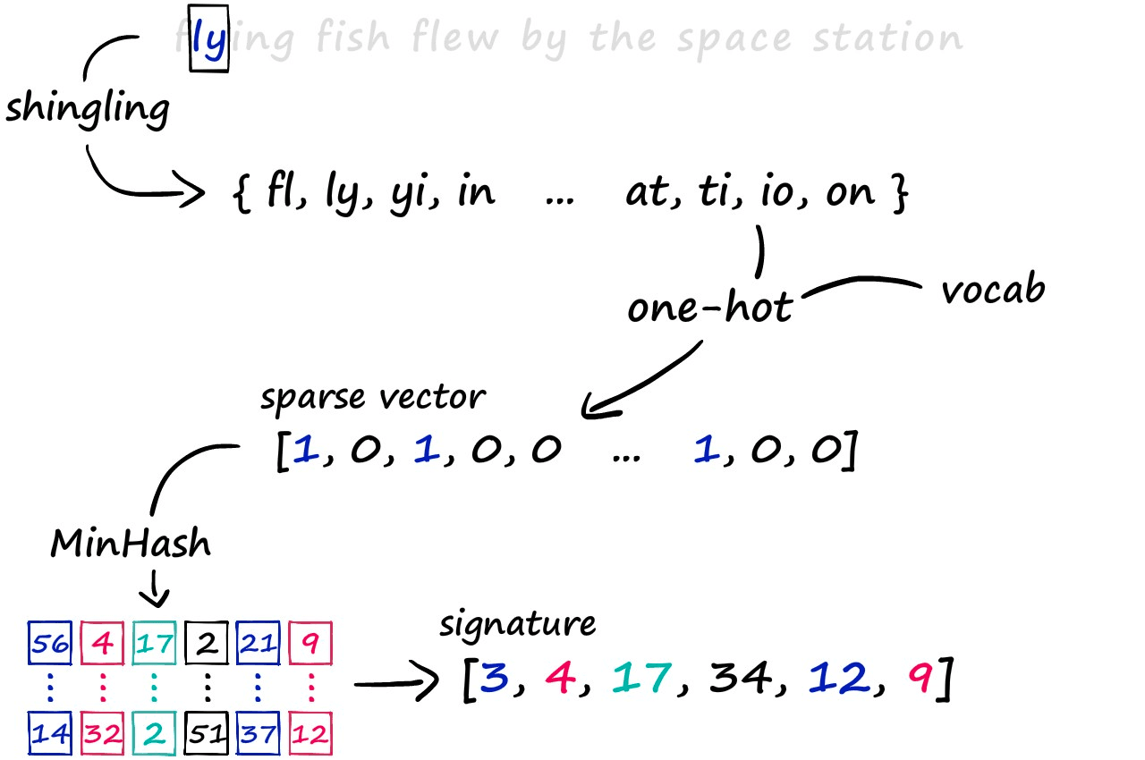
The LSH approach we’re exploring consists of a three-step process. First, we convert text to sparse vectors using k-shingling (and one-hot encoding), then use minhashing to create ‘signatures’ — which are passed onto our LSH process to weed out candidate pairs.
We will discuss some of the other LSH methods in future articles. But for now, let’s work through the traditional process in more depth.
k-Shingling
k-Shingling, or simply shingling — is the process of converting a string of text into a set of ‘shingles’. The process is similar to moving a window of length k down our string of text and taking a picture at each step. We collate all of those pictures to create our set of shingles.
Shingling also removes duplicate items (hence the word ‘set’). We can create a simple k-shingling function in Python like so:
a = "flying fish flew by the space station"
b = "we will not allow you to bring your pet armadillo along"
c = "he figured a few sticks of dynamite were easier than a fishing pole to catch fish"def shingle(text: str, k: int):
shingle_set = []
for i in range(len(text) - k+1):
shingle_set.append(text[i:i+k])
return set(shingle_set)a = shingle(a, k)
b = shingle(b, k)
c = shingle(c, k)
print(a){'y ', 'pa', 'ng', 'yi', 'st', 'sp', 'ew', 'ce', 'th', 'sh', 'fe', 'e ', 'ta', 'fl', ' b', 'in', 'w ', ' s', ' t', 'he', ' f', 'ti', 'fi', 'is', 'on', 'ly', 'g ', 'at', 'by', 'h ', 'ac', 'io'}
And with this, we have our shingles. Next, we create our sparse vectors. To do this, we first need to union all of our sets to create one big set containing all of the shingles across all of our sets — we call this the vocabulary (or vocab).
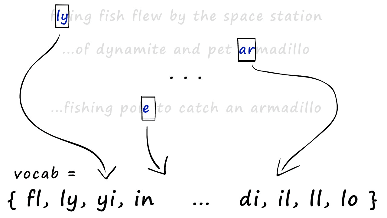
We use this vocab to create our sparse vector representations of each set. All we do is create an empty vector full of zeros and the same length as our vocab — then, we look at which shingles appear in our set.
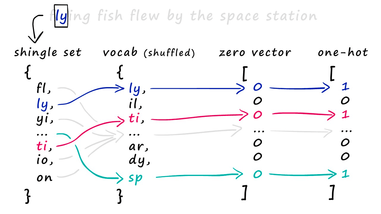
For every shingle that appears, we identify the position of that shingle in our vocab and set the respective position in our new zero-vector to 1. Some of you may recognize this as one-hot encoding.
Minhashing
Minhashing is the next step in our process, allowing us to convert our sparse vectors into dense vectors. Now, as a pre-warning — this part of the process can seem confusing initially — but it’s very simple once you get it.
We have our sparse vectors, and what we do is randomly generate one minhash function for every position in our signature (e.g., the dense vector).
So, if we wanted to create a dense vector/signature of 20 numbers — we would use 20 minhash functions.
Now, those MinHash functions are simply a randomized order of numbers — and we count from 1 to the final number (which is len(vocab)). Because the order of these numbers has been randomized, we may find that number *1 *is in position 57 (for example) of our randomized MinHash function.
Above, we’re using a smaller vocab containing six values so we can easily visualize the process.
We look at our sparse vector and say, “did this shingle at vocab[1] exist in our set?”. If it did — the sparse vector value will be 1 — in this case, it did not exist (hence the 0 value). So, we move to number 2, identify its position (0) and ask the same question. This time, the answer is yes, and so our minhash output is 2.
That’s how we produce one value in our minhash signature. But we need to produce 20 (or more) of these values. So, we assign a different minhash function to each signature position — and repeat the process.
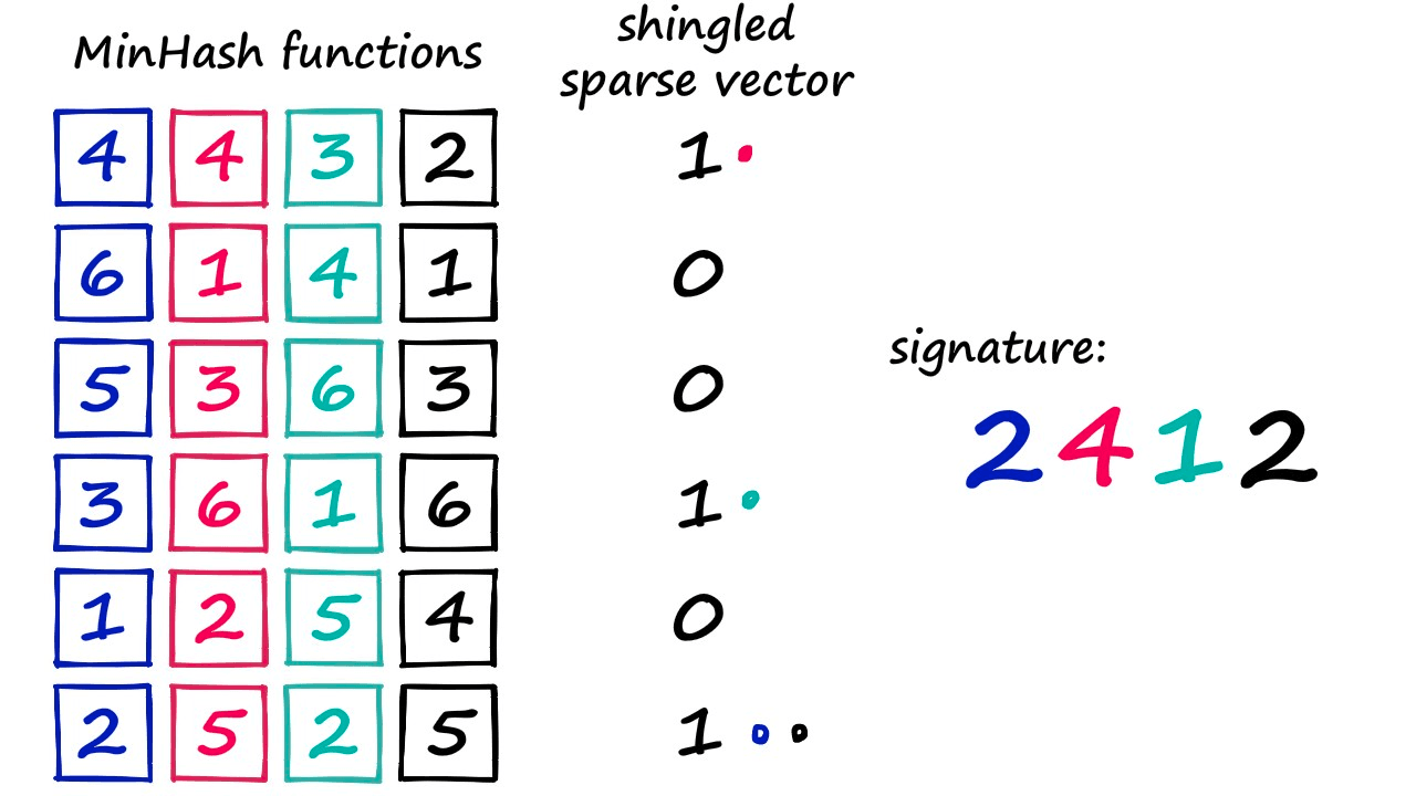
At the end of this, we produce our minhash signature — or dense vector.
Let’s go ahead and write that in code. We have three steps:
1. Generate a randomized MinHash vector.**
hash_ex = list(range(1, len(vocab)+1))
print(hash_ex) # we haven't shuffled yet[1, 2, 3, 4, 5 ... 99, 100, 101, 102]
from random import shuffle

shuffle(hash_ex)
print(hash_ex)[63, 7, 94, 16, 36 ... 6, 55, 80, 56]
2. Loop through this randomized MinHash vector (starting at 1), and match the index of each value to the equivalent values in the sparse vector a_1hot. If we find a 1 — that index is our signature value.
print(f"7 -> {hash_ex.index(7)}"). # note that value 7 can be found at index 1 in hash_ex7 -> 1
We now have a randomized list of integers which we can use in creating our *hashed* signatures. What we do now is begin counting from `1` through to `len(vocab) + 1`, extracting the position of this number in our new `hash_ex` list, like so:for i in range(1, 5):
print(f"{i} -> {hash_ex.index(i)}")1 -> 58
2 -> 19
3 -> 96
4 -> 92
What we do with this is count up from `1` to `len(vocab) + 1` and find if the resultant `hash_ex.index(i)` position in our one-hot encoded vectors contains a positive value (`1`) in that position, like so:for i in range(1, len(vocab)+1):
idx = hash_ex.index(i)
signature_val = a_1hot[idx]
print(f"{i} -> {idx} -> {signature_val}")
if signature_val == 1:
print('match!')
break1 -> 58 -> 0
2 -> 19 -> 0
3 -> 96 -> 0
4 -> 92 -> 0
5 -> 83 -> 0
6 -> 98 -> 1
match!
3. Build a signature from multiple iterations of 1 and 2 (we’ll formalize the code from above into a few easier to use functions):
def create_hash_func(size: int):
    # function for creating the hash vector/function
    hash_ex = list(range(1, len(vocab)+1))
    shuffle(hash_ex)
    return hash_ex

def build_minhash_func(vocab_size: int, nbits: int):
    # function for building multiple minhash vectors
    hashes = []
    for _ in range(nbits):
        hashes.append(create_hash_func(vocab_size))
    return hashes

# we create 20 minhash vectors
minhash_func = build_minhash_func(len(vocab), 20)def create_hash(vector: list):
# use this function for creating our signatures (eg the matching)
signature = []
for func in minhash_func:
for i in range(1, len(vocab)+1):
idx = func.index(i)
signature_val = vector[idx]
if signature_val == 1:
signature.append(idx)
break
return signature# now create signatures
a_sig = create_hash(a_1hot)
b_sig = create_hash(b_1hot)
c_sig = create_hash(c_1hot)
print(a_sig)
print(b_sig)[44, 21, 73, 14, 2, 13, 62, 70, 17, 5, 12, 86, 21, 18, 10, 10, 86, 47, 17, 78]
[97, 96, 57, 82, 43, 67, 75, 24, 49, 28, 67, 56, 96, 18, 11, 85, 86, 19, 65, 75]
And that is MinHashing — it’s really nothing more complex than that. We’ve taken a sparse vector and compressed it into a more densely packed, 20-number signature.
Information Transfer from Sparse to Signature
Is the information truly maintained between our much larger sparse vector and much smaller dense vector? It’s not easy for us to visually identify a pattern in these new dense vectors — but we can calculate the similarity between vectors.
If the information truly has been retained during our downsizing — surely the similarity between vectors will be similar too?
Well, we can test that. We use Jaccard similarity to calculate the similarity between our sentences in shingle format — then repeat for the same vectors in signature format:
def jaccard(a: set, b: set):
return len(a.intersection(b)) / len(a.union(b))jaccard(a, b), jaccard(set(a_sig), set(b_sig))(0.14814814814814814, 0.10344827586206896)jaccard(a, c), jaccard(set(a_sig), set(c_sig))(0.22093023255813954, 0.13793103448275862)We see pretty close similarity scores for both — so it seems that the information is retained. Let’s try again for b and c:
jaccard(b, c), jaccard(set(b_sig), set(c_sig))(0.45652173913043476, 0.34615384615384615)Here we find much higher similarity, as we would expect — it looks like the similarity information is maintained between our sparse vectors and signatures! So, we’re now fully prepared to move onto the LSH process.
Band and Hash
The final step in identifying similar sentences is the LSH function itself.
We will be taking the banding approach to LSH — which we could describe as the traditional method. It will be taking our signatures, hashing segments of each signature, and looking for hash collisions — as we described earlier in the article.
Through this method, we produce these vectors of equal length that contain positive integer values in the range of 1 → len(vocab) — these are the signatures that we typically input into this LSH algorithm.
Now, if we were to hash each of these vectors as a whole, we may struggle to build a hashing function that accurately identifies similarity between them — we don’t require that the full vector is equal, only that parts of it are similar.
In most cases, even though parts of two vectors may match perfectly — if the remainder of the vectors are not equal, the function will likely hash them into separate buckets.
We don’t want this. We want signatures that share even some similarity to be hashed into the same bucket , thus being identified as candidate pairs.
How it Works
The banding method solves this problem by splitting our vectors into sub-parts called bands b. Then, rather than processing the full vector through our hash function, we pass each band of our vector through a hash function.
Imagine we split a 100-dimensionality vector into 20 bands. That gives us 20 opportunities to identify matching sub-vectors between our vectors.
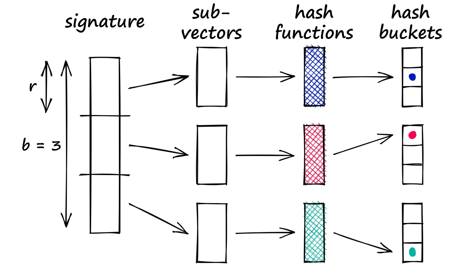
We can now add a more flexible condition — given a collision between any two sub-vectors, we consider the respective full vectors as candidate pairs.
Now, only part of the two vectors must match for us to consider them. But of course, this also increases the number of false positives (samples that we mark as candidate matches where they are not similar). However, we do try to minimize these as far as possible.
We can implement a simple version of this. First, we start by splitting our signature vectors a, b, and c:
def split_vector(signature, b):
    assert len(signature) % b == 0
    r = int(len(signature) / b)
    # code splitting signature in b parts
    subvecs = []
    for i in range(0, len(signature), r):
        subvecs.append(signature[i : i+r])
    return subvecs
Split into 10 bands, creating rows of `2`
band_a = split_vector(a_sig, 10)
band_b = split_vector(b_sig, 10)
band_b[[42, 43],
[69, 55],
[29, 96],
[86, 46],
[92, 5],
[72, 65],
[29, 5],
[53, 33],
[40, 94],
[96, 70]]band_c = split_vector(c_sig, 10)
band_c[[90, 43],
[69, 55],
[4, 101],
[35, 15],
[92, 22],
[18, 65],
[40, 18],
[53, 33],
[40, 94],
[80, 14]]Then we loop through the lists to identify any matches between sub-vectors. If we find any matches — we take those vectors as candidate pairs.
for b_rows, c_rows in zip(band_b, band_c):
    if b_rows == c_rows:
        print(f"Candidate pair: {b_rows} == {c_rows}")
        # we only need one band to match
breakCandidate pair: [69, 55] == [69, 55]
And let's do the same for **a**.for a_rows, b_rows in zip(band_a, band_b):
if a_rows == b_rows:
print(f"Candidate pair: {a_rows} == {b_rows}")
# we only need one band to match
breakfor a_rows, c_rows in zip(band_a, band_c):
if a_rows == c_rows:
print(f"Candidate pair: {b_rows} == {c_rows}")
# we only need one band to match
breakWe find that our two more similar sentences, b, and **c **— are identified as candidate pairs. The less similar of the trio, a — is not identified as a candidate. This is a good result, but if we want to really test LSH, we will need to work with more data.
Testing LSH
What we have built thus far is a very inefficient implementation — if you want to implement LSH, this is certainly not the way to do it. Rather, use a library built for similarity search — like Faiss, or a managed solution like Pinecone.
But working through the code like this should — if nothing else — make it clear how LSH works. However, we will now be replicating this for much more data, so we will rewrite what we have so far using Numpy.
The code will function in the same way — and you can find each of the functions (alongside explanations) in this notebook.
Getting Data
First, we need to get data. There is a great repository here that contains several datasets built for similarity search testing. We will be extracting a set of sentences from here.
import requests
import pandas as pd
import io

url = "https://raw.githubusercontent.com/brmson/dataset-sts/master/data/sts/sick2014/SICK_train.txt"

text = requests.get(url).text

data = pd.read_csv(io.StringIO(text), sep='\t')
data.head() pair_ID sentence_A \
0 1 A group of kids is playing in a yard and an ol...
1 2 A group of children is playing in the house an...
2 3 The young boys are playing outdoors and the ma...
3 5 The kids are playing outdoors near a man with ...
4 9 The young boys are playing outdoors and the ma...
sentence_B relatedness_score \
0 A group of boys in a yard is playing and a man... 4.5
1 A group of kids is playing in a yard and an ol... 3.2
2 The kids are playing outdoors near a man with ... 4.7
3 A group of kids is playing in a yard and an ol... 3.4
4 A group of kids is playing in a yard and an ol... 3.7
entailment_judgment
0 NEUTRAL
1 NEUTRAL
2 ENTAILMENT
3 NEUTRAL
4 NEUTRAL sentences = data['sentence_A'].tolist()
sentences[:3]['A group of kids is playing in a yard and an old man is standing in the background',
'A group of children is playing in the house and there is no man standing in the background',
'The young boys are playing outdoors and the man is smiling nearby']Shingles
Once we have our data, we can create our one-hot encodings — this time stored as a NumPy array (find full code and functions here).
k = 8  # shingle size

# build shingles
shingles = []
for sentence in sentences:
    shingles.append(build_shingles(sentence, k))

# build vocab
vocab = build_vocab(shingles)

# one-hot encode our shingles
shingles_1hot = []
for shingle_set in shingles:
    shingles_1hot.append(one_hot(shingle_set, vocab))
# stack into single numpy array
shingles_1hot = np.stack(shingles_1hot)
shingles_1hot.shape(4500, 36466)shingles_1hot[:5]array([[0., 0., 0., ..., 0., 0., 0.],
[0., 0., 0., ..., 0., 0., 0.],
[0., 0., 0., ..., 0., 0., 0.],
[0., 0., 0., ..., 0., 0., 0.],
[0., 0., 0., ..., 0., 0., 0.]])sum(shingles_1hot[0]) # confirm we have 1s73.0Now we have our one-hot encodings. The shingles_1hot array contains *4500 *sparse vectors, where each vector is of length 36466.
MinHashing
As before, we will compress our sparse vectors into dense vector ‘signatures’ with minhashing. Again, we will be using our NumPy implementation, which you can find the full code here.
arr = minhash_arr(vocab, 100)

signatures = []

for vector in shingles_1hot:
    signatures.append(get_signature(arr, vector))

# merge signatures into single array
signatures = np.stack(signatures)
signatures.shape(4500, 100)signatures[0]array([ 65, 438, 534, 1661, 1116, 200, 1206, 583, 141, 766, 92,
52, 7, 287, 587, 65, 135, 581, 136, 838, 1293, 706,
31, 414, 374, 837, 72, 1271, 872, 1136, 201, 1109, 409,
384, 405, 293, 279, 901, 11, 904, 1480, 763, 1610, 518,
184, 398, 128, 49, 910, 902, 263, 80, 608, 69, 185,
1148, 1004, 90, 547, 1527, 139, 279, 1063, 646, 156, 357,
165, 6, 63, 269, 103, 52, 55, 908, 572, 613, 213,
932, 244, 64, 178, 372, 115, 427, 244, 263, 944, 148,
55, 63, 232, 1266, 371, 289, 107, 413, 563, 613, 65,
188])We’ve compressed our sparse vectors from a length of 36466 to signatures of length 100. A big difference, but as we demonstrated earlier, this compression technique retains similarity information very well.
LSH
Finally, onto the LSH portion. We will use a Python dictionary here to hash and store our candidate pairs — again. The full code is here.
b = 20

lsh = LSH(b)

for signature in signatures:
lsh.add_hash(signature)lsh.buckets[{'65,438,534,1661,1116': [0],
'65,2199,534,806,1481': [1],
'312,331,534,1714,575': [2, 4],
'941,331,534,466,75': [3],
...
'5342,1310,335,566,211': [1443, 1444],
'1365,722,3656,1857,1023': [1445],
'393,858,2770,1799,772': [1446],
...}]It’s important to note that our lsh.buckets variable actually contains a separate dictionary for each band — we do not mix buckets between different bands.
We see in our buckets the vector IDs (row numbers) , so all we need to do to extract our candidate pairs is loop through all buckets and extract pairs.
candidate_pairs = lsh.check_candidates()
len(candidate_pairs)7243list(candidate_pairs)[:5][(1646, 1687), (3234, 3247), (1763, 2235), (2470, 2622), (3877, 3878)]After identifying our candidate pairs, we would restrict our similarity calculations to those pairs only — we will find that some will be within our similarity threshold, and others will not.
The objective here is to restrict our scope and reduce search complexity while still maintaining high accuracy in identifying pairs.
We can visualize our performance here by measuring the candidate pair classification (1 or 0) against actual cosine (or Jaccard) similarity.
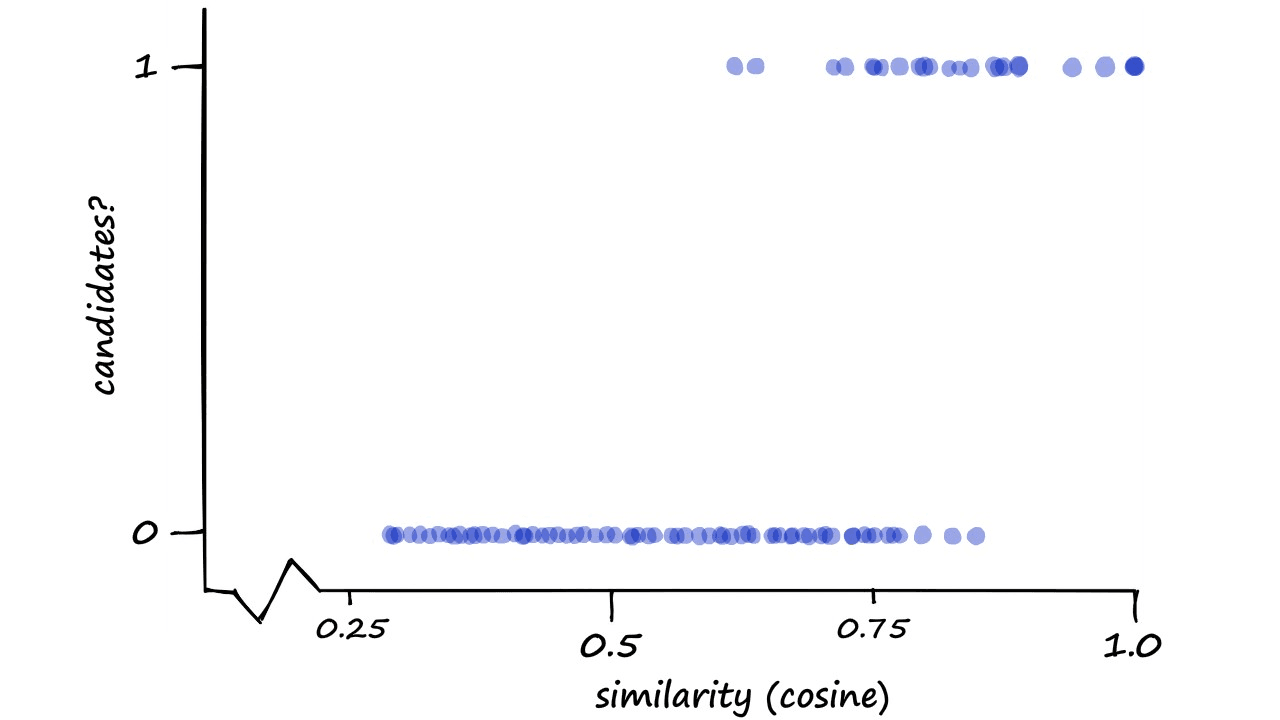
Now, this may seem like a strange way to visualize our performance — and you are correct, it is — but we do have a reason.
Optimizing the Bands
It is possible to optimize our band value b to shift the similarity threshold of our LSH function. The similarity threshold is the point at which we would like our LSH function to switch from a non-candidate to a candidate pair.
We formalize this probability-similarity relationship as so:

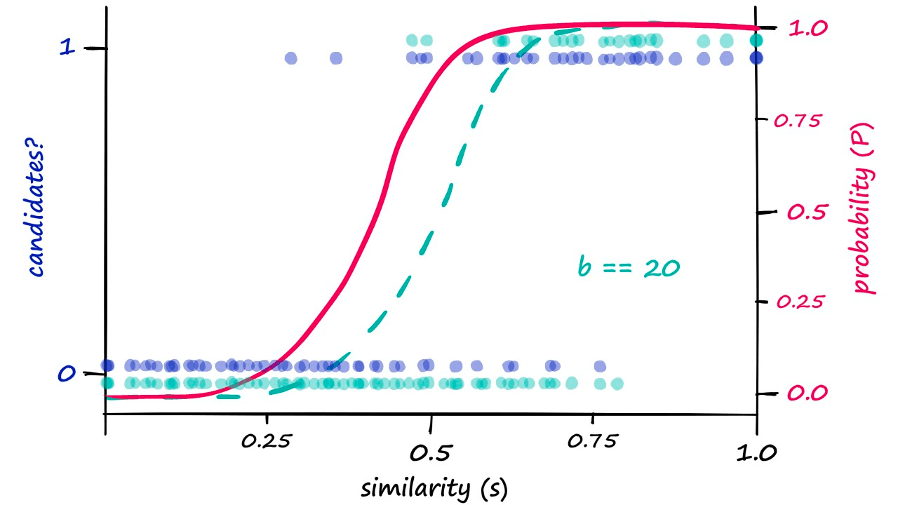
Now, if we were to visualize this probability-similarity relationship for our current b and r values we should notice a pattern:
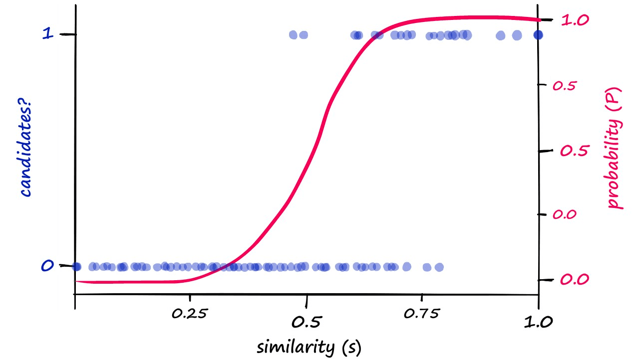
Although the alignment isn’t perfect, we can see a correlation between the theoretical, calculated probability — and the genuine candidate pair results. Now, we can push the probability of returning candidate-pairs at different similarity scores left or right by modifying b:
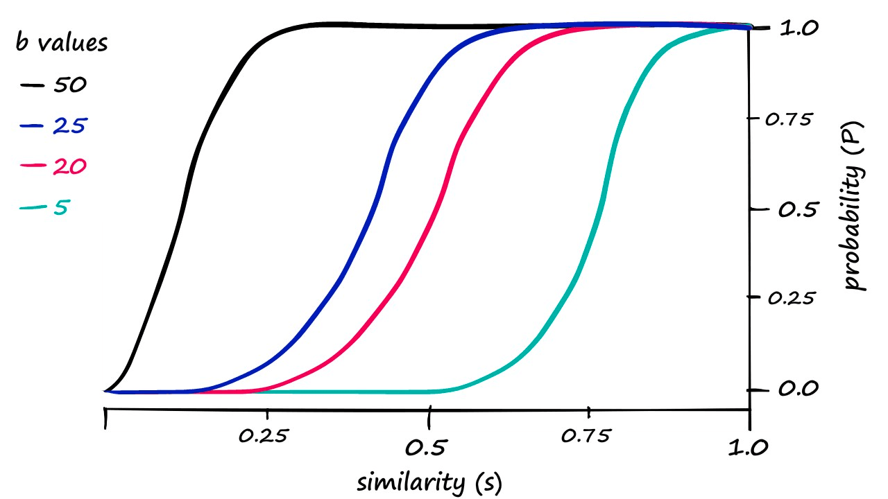
These are our calculated probability values. If we decided that our previous results where b == 20 required too high a similarity to count pairs as candidate pairs — we would attempt to shift the similarity threshold to the left.
Looking at this graph, a b value of 25 looks like it could shift our genuine results just enough. So, let’s visualize our results when using b == 25:
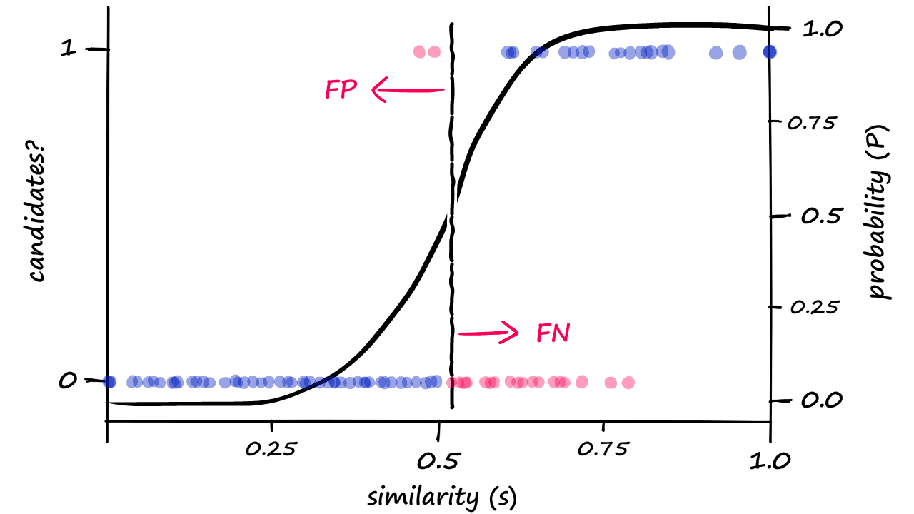
Because we are now returning more candidate pairs, this will naturally result in more false positives — where we return ‘candidate pair’ for dissimilar vectors. This is an unavoidable consequence of modifying b, which we can visualize as:
Great! We’ve built our LSH process from scratch — and even managed to tune our similarity threshold.
That’s everything for this article on the principles of LSH. Not only have we covered LSH, but also shingling and the MinHash function!
In practice, we would most likely want to implement LSH using libraries built specifically for similarity search. We will be covering LSH — specifically the random projection method — in much more detail, alongside its implementation in Faiss.
However, if you’d prefer a quick rundown of some of the key indexes (and their implementations) in similarity search, we cover them all in our overview of vector indexes.
Further Resources
- Jupyter Notebooks
- J. Ullman et al., Mining of Massive Datasets
Was this article helpful?