Zero Shot Object Detection with OpenAI's CLIP
The Imagenet Large Scale Visual Recognition Challenge (ILSVRC)[1] was a world-changing competition hosted annually from 2010 until 2017. During this time, the competition acted as the catalyst for the explosion of deep learning[2] and was the place to find state-of-the-art image classification, object localization, and object detection.
Researchers fine-tuned better-performance computer vision (CV) models to achieve ever more impressive results year-after-year. But there was an unquestioned assumption causing problems.
We assumed that every new task required model fine-tuning, this required a lot of data, and this needed both time and capital.
It wasn’t until very recently that this assumption was questioned and proven wrong.
The astonishing rise of multi-modal models has made the impossible possible across various domains and tasks. One of those is zero-shot object detection and localization.
“Zero-shot” means applying a model without the need for fine-tuning. Meaning we take a multi-modal model and use it to detect images in one domain, then switch to another entirely different domain without the model seeing a single training example from the new domain.
Not needing a single training example means we completely skip the hard part of data annotation and model training. We can focus solely on application of our models.
In this chapter, we will explore how to apply OpenAI’s CLIP to this task—using CLIP for localization and detection across domains with zero fine-tuning.
Classification, Localization, and Detection
Image classification is one of the most straightforward tasks in visual recognition and the first step on the way to object detection. It consists of assigning a categorical label to an image.
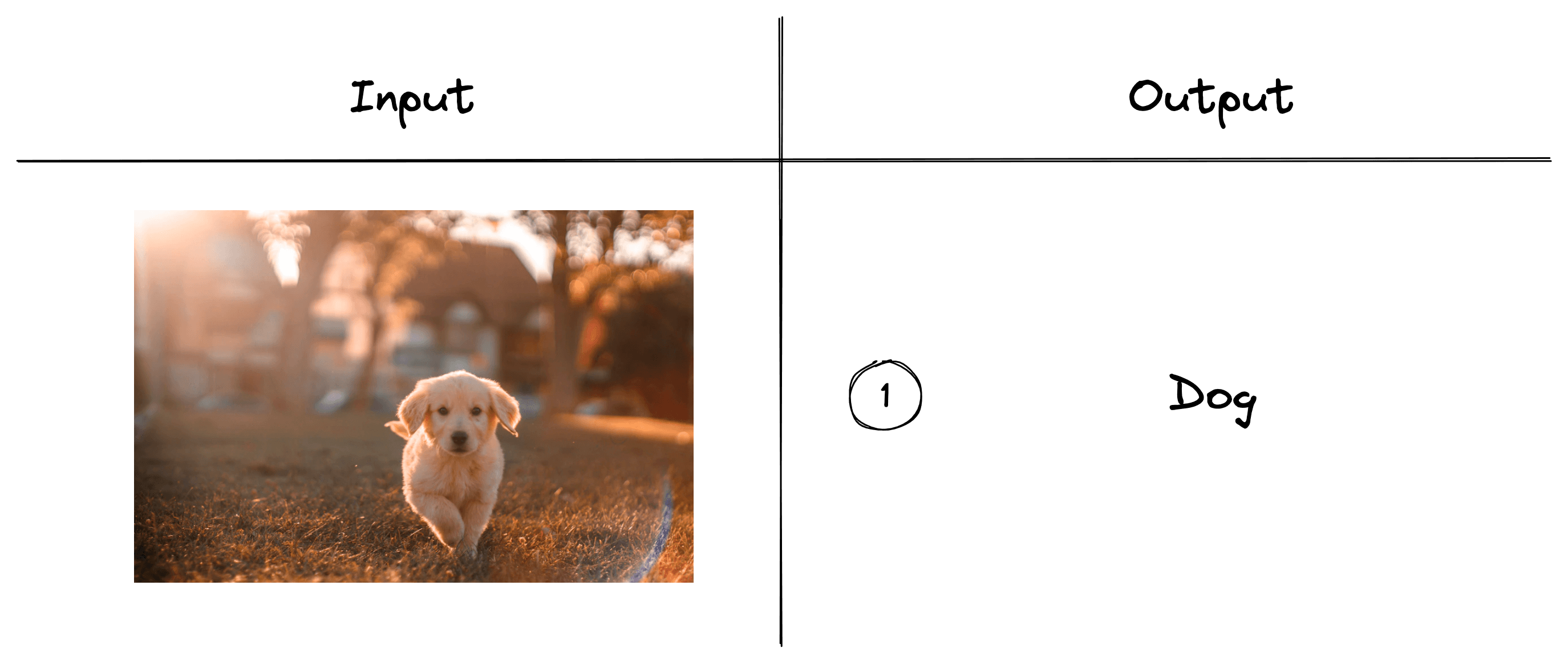
We could have an image classification model that identifies animals and could classify images of dogs, cats, mice, etc. If we pass the above image into this model, we’d expect it to return the class “dog”.
Object localization takes this one step further by “localizing” the identified object.
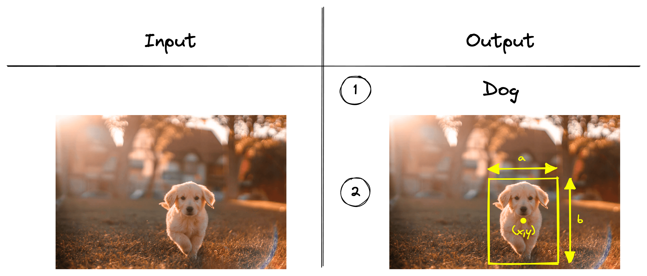
When we localize the object, we identify the object’s coordinates on the image. That typically includes a set of patches where the object is located or a bounding box defined by () coordinates, box width, and box height.
Object detection can be thought of as the next step. With detection, we are localizing multiple object instances within the same image.
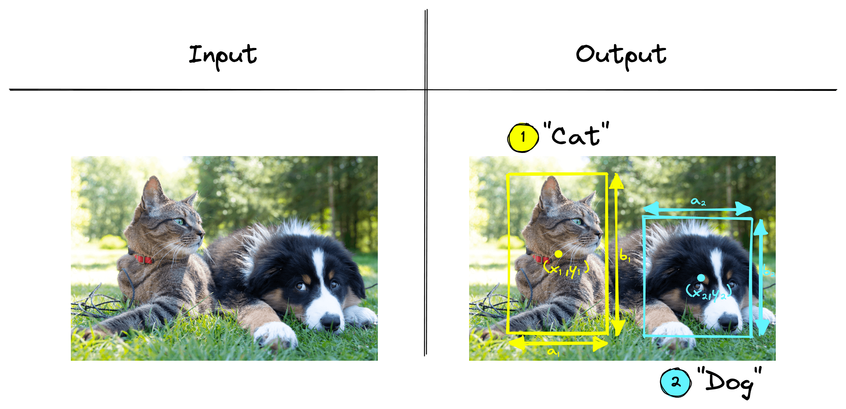
In the example above, we are detecting two different objects within the image, a cat and a dog. Both objects are localized, and the results are returned.
Object detection can also identify multiple instances of the same object in a single image. If we added another dog to the previous image, an object detection algorithm could detect two dogs and a single cat.
Zero Shot CLIP
OpenAI’s CLIP is a multi-modal model pretrained on a massive dataset of text-image pairs [3]. It can identify text and images with similar meanings by encoding both modalities into a shared vector space.
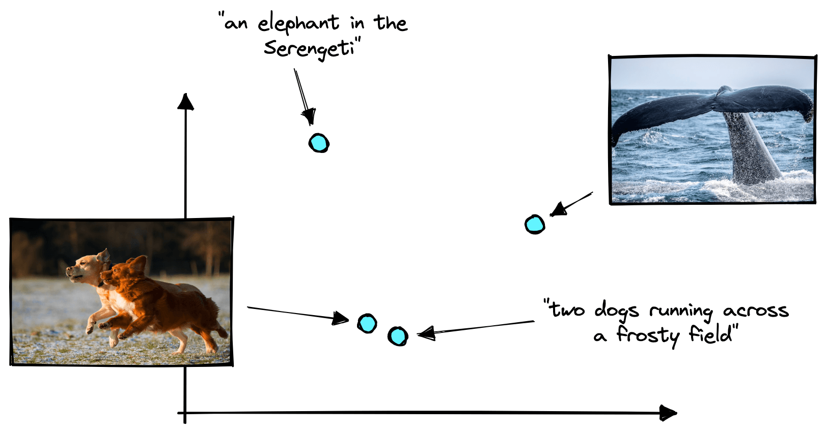
CLIP’s broad pretraining means it can perform effectively across many domains. We can adjust the task being performed (i.e. from classification to detection) with just a few lines of code. A big part of this flexibility if thanks to the multi-modal vector embeddings built by CLIP.
These vector embeddings allow us to switch from text-to-image search, image classification, and object detection. We simply adjust how we preprocess data being fed into CLIP, or how we interpret the similarity scores between the CLIP embeddings. The model itself requires no modification.
For classification, we need to give CLIP a list of our class labels, and it will encode them into a vector space:
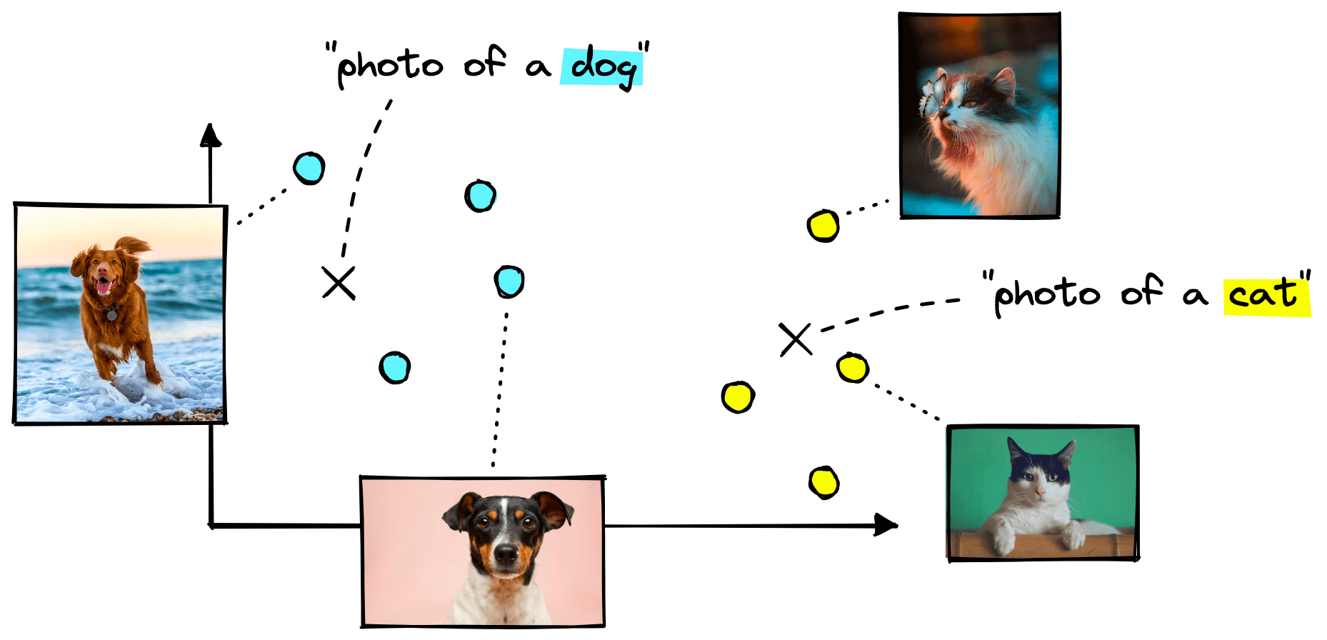
From there, we give CLIP the images we’d like to classify. CLIP will encode them in the same vector space, and we find which of the class label embeddings is nearest to our image embeddings.
Object Localization
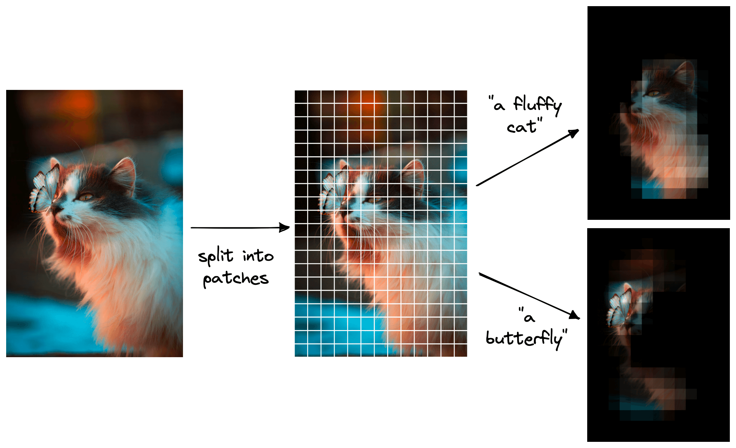
We can apply similar logic to using CLIP in a zero-shot object localization setting. As before, we create a class label embedding like "a fluffy cat". But, unlike before, we don’t feed the entire image into CLIP.
To localize an object, we break the image into many small patches. We then pass a window over these patches, moving across the entire image and generating an image embedding for a unique window.
We can calculate the similarity between these patch image embeddings and our class label embeddings — returning a score for each patch.
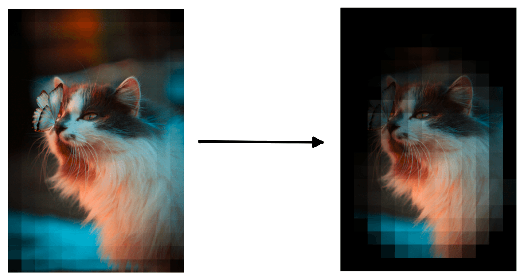
After calculating the similarity scores for every patch, we collate them into a map of relevance across the entire image. We use that “map” to identify the location of the object of interest.
From there, we can recreate the traditional approach of creating a “bounding box” around the object.
Both of these visuals capture the same information but displays them in different ways.
Occlusion Algorithm
Occlusion is another method of localization where we slide a black patch across the image. The idea being that we dentify similarity by the “absence” of an object [4][5].
If the black patch covers the object we are looking for, the similarity score will drop. We then take that position as the assumed location of our object.
Object Detection
There is a fine line between object localization and object detection. With object localization, we perform a “classification” of a single object followed by the localization of that object. With object detection, we perform localization for multiple classes and/or objects.
With our cat and butterfly image, we could search for two objects; "a fluffy cat" and "a butterfly". We use object localization to identify each individual object, but by iteratively identifying multiple objects, this becomes object detection.
We stick with the bounding box visualizations for object detection, as the other method makes it harder to visualize multiple objects within the same image.
We have covered the idea behind object localization and detection in a zero-shot setting with CLIP. Now let’s take a look at how to implement it.
Detection with CLIP
Before we move on to any classification, localization, or detection task, we need images to process. We will use a small demo dataset named jamescalam/image-text-demo hosted on Hugging Face datasets.
# import dataset
from datasets import load_dataset

data = load_dataset(
    "jamescalam/image-text-demo",
    split="train",
    revision="180fdae"
)
dataDataset({
features: ['text', 'image'],
num_rows: 21
})The dataset contains the image of a butterfly landing on a cat’s nose. We can view it in a Jupyter notebook with the following:
data[2]['image']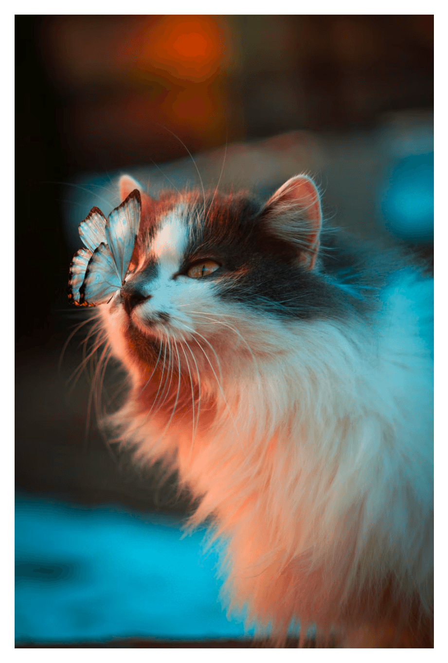
We have downloaded the image, but it is not in the format we need for localization. For that, we must break the image into smaller patches.
Creating Patches
To create the patches, we must first convert our PIL image object into a PyTorch tensor. We can do this using torchvision.transforms.
from torchvision import transforms

# transform the image into tensor
transt = transforms.ToTensor()

img = transt(data[2]["image"])
img.data.shapetorch.Size([3, 5184, 3456])Our tensor has 3 color channels (RGB), a height of 5184 pixels, and width of 3456 pixels.
Assuming each patch has an equal height and width of 256 pixels, we must reshape this tensor into a tensor of shape (1, 20, 13, 3, 256, 256) where 20 and 13 of the number of patches in height and width of the image and 1 represents the batch dimension.
We first add the batch dimension and move the color channels' dimension behind the height and width dimensions.
# add batch dimension and shift color channels
patches = img.data.unfold(0,3,3)
patches.shapetorch.Size([1, 5184, 3456, 3])Following this, we broke up the image into horizontal patches first. All patches will be square with dimensionalities of 256x256, so the horizontal patch height equals 256 pixels.
# break the image into patches (in height dimension)
patch = 256

patches = patches.unfold(1, patch, patch)
patches.shapetorch.Size([1, 20, 3456, 3, 256])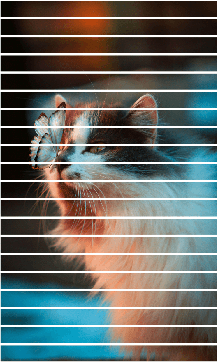
We need one more unfold to create the vertical space between patches.
# break the image into patches (in width dimension)
patches = patches.unfold(2, patch, patch)
patches.shapetorch.Size([1, 20, 13, 3, 256, 256])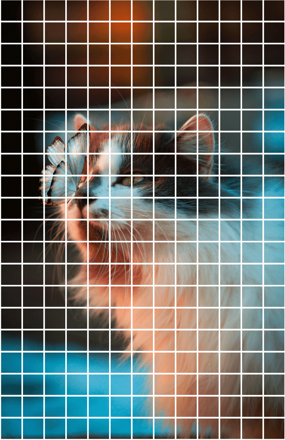
Every patch is tiny, and looking at a single patch gives us little-to-no information about the image’s content. Rather than feeding single patches to CLIP, we merge multiple patches to create a big patch passed to CLIP.
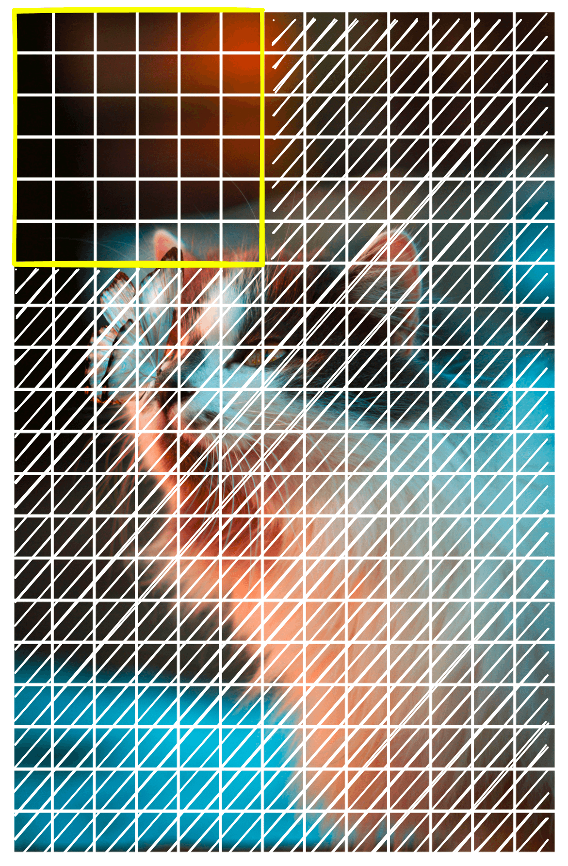
We call this grouping of patches a window. A larger window size captures more global views of the image, whereas a smaller window can produce a more precise map at the risk of missing larger objects. To slide across the image and create a big_batch at each step, we do the following:
window = 6
stride = 1

# window slides from top to bottom
for Y in range(0, patches.shape[1]-window+1, stride):
    # window slides from left to right
    for X in range(0, patches.shape[2]-window+1, stride):
        # initialize an empty big_patch array
        big_patch = torch.zeros(patch*window, patch*window, 3)
        # this gets the current batch of patches that will make big_batch
        patch_batch = patches[0, Y:Y+window, X:X+window]
        # loop through each patch in current batch
        for y in range(patch_batch.shape[1]):
            for x in range(patch_batch.shape[0]):
                # add patch to big_patch
                big_patch[
                    y*patch:(y+1)*patch, x*patch:(x+1)*patch, :
                ] = patch_batch[y, x].permute(1, 2, 0)
        # display current big_patch
        plt.imshow(big_patch)
plt.show()We will re-use this logic later when creating our patch image embeddings. Before we do that, we must initialize CLIP.
CLIP and Localization
The Hugging Face transformers library contains an implementation of CLIP named openai/clip-vit-base-patch32. We can download and initialize it like so:
from transformers import CLIPProcessor, CLIPModel
import torch

# define processor and model
model_id = "openai/clip-vit-base-patch32"

processor = CLIPProcessor.from_pretrained(model_id)
model = CLIPModel.from_pretrained(model_id)

# move model to device if possible
device = 'cuda' if torch.cuda.is_available() else 'cpu'

model.to(device)
Note that we also move to model to a CUDA-enabled GPU if possible to reduce inference times.
With CLIP initialized, we can rerun the patch sliding logic, but this time we will calculate the similarity between each big_patch and the text label "a fluffy cat".
window = 6
stride = 1

scores = torch.zeros(patches.shape[1], patches.shape[2])
runs = torch.ones(patches.shape[1], patches.shape[2])

for Y in range(0, patches.shape[1]-window+1, stride):
    for X in range(0, patches.shape[2]-window+1, stride):
        big_patch = torch.zeros(patch*window, patch*window, 3)
        patch_batch = patches[0, Y:Y+window, X:X+window]
        for y in range(window):
            for x in range(window):
                big_patch[
                    y*patch:(y+1)*patch, x*patch:(x+1)*patch, :
                ] = patch_batch[y, x].permute(1, 2, 0)
        # we preprocess the image and class label with the CLIP processor
        inputs = processor(
            images=big_patch,  # big patch image sent to CLIP
            return_tensors="pt",  # tell CLIP to return pytorch tensor
            text="a fluffy cat",  # class label sent to CLIP
            padding=True
        ).to(device) # move to device if possible

        # calculate and retrieve similarity score
        score = model(**inputs).logits_per_image.item()
        # sum up similarity scores from current and previous big patches
        # that were calculated for patches within the current window
        scores[Y:Y+window, X:X+window] += score
        # calculate the number of runs on each patch within the current window
        runs[Y:Y+window, X:X+window] += 1
Here we have also added scores and runs that we will use to calculate the mean score for each patch. We calculate the scores tensor as the sum of every big_patch score calculated while the patches were within the window.
Some patches will be seen more often than others (for example, the top-left patch is seen once), so the scores will be much greater for patches viewed more frequently. That is why we use the runs tensor to keep track of the “visit frequency” for each patch. With both tensors populated, we calculate the mean score:
scores /= runsThe scores tensor typically contains a smooth gradient of values as a byproduct of the scoring function sliding over each window. This means the scores gradually fade to 0.0 the further they are from the object of interest.
We cannot accurately visualize the object location with the current scores. Ideally, we should push low scores to zero while maintaining a range of values for higher scores. We can do this by clipping our outputs and normalizing the remaining values.
# clip the scores
scores = np.clip(scores-scores.mean(), 0, np.inf)

# normalize scores
scores = (
    scores - scores.min()) / (scores.max() - scores.min()
)
With that, our patch scores are ready, and we can move on to visualizing the results.
Visualize Localization
Each patch in the (20,13)(20,13) patches tensor is assigned a similarity score within the range of 00 (not similar) to 11 (perfect match).
If we can align the scores with the original image pixels, we can multiply each pixel by its corresponding similarity score. Those near 00 will be dark, and near 11 will maintain their original brightness.
The only problem is that these two tensors are not the same shape:
scores.shape, patches.shape[Out]: (torch.Size([20, 13]), torch.Size([1, 20, 13, 3, 256, 256]))
We need to reshape patches to align with scores. To do that, we use squeeze to remove the batch dimension at position 0 and then re-order the dimensions using permute.
# transform the patches tensor
adj_patches = patches.squeeze(0).permute(3, 4, 2, 0, 1)
adj_patches.shape
[Out]: torch.Size([256, 256, 3, 20, 13])
From there, we multiply the adjusted patches and scores to return the brightness-adjusted patches. These need to be permuted again to be visualized with matplotlib.
# multiply patches by scores
adj_patches = adj_patches * scores

# rotate patches to visualize
adj_patches = adj_patches.permute(3, 4, 2, 0, 1)
adj_patches.shape
[Out]: torch.Size([20, 13, 3, 256, 256])
Now we’re ready to visualize:
Y = adj_patches.shape[0]
X = adj_patches.shape[1]

fig, ax = plt.subplots(Y, X, figsize=(X*.5, Y*.5))
for y in range(Y):
    for x in range(X):
        ax[y, x].imshow(adj_patches[y, x].permute(1, 2, 0))
        ax[y, x].axis("off")
        ax[y, x].set_aspect('equal')
plt.subplots_adjust(wspace=0, hspace=0)
plt.show()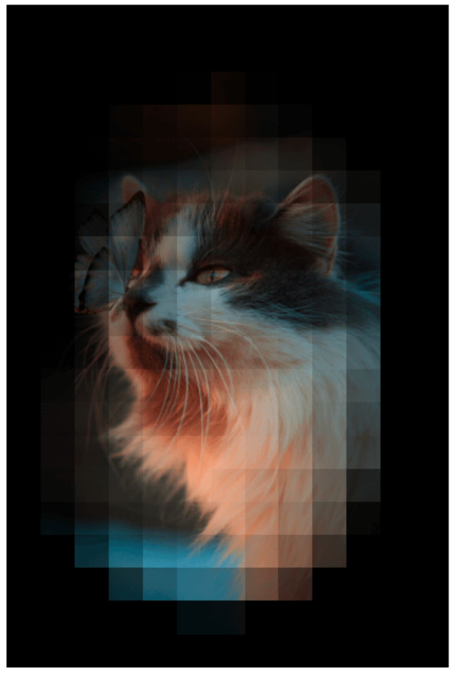
That works well. We can repeat the same but with the prompt "a butterfly" to return:
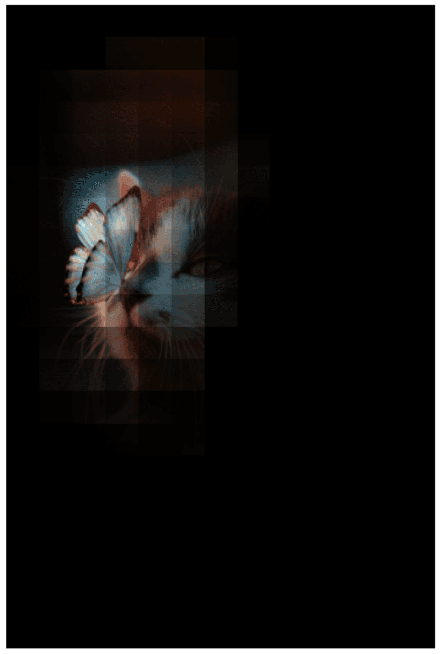
CLIP shows another good result and demonstrates how easy it is to add new labels to classification and localization tasks with CLIP.
Bounding Box
Before moving on to object detection, we need to rework the visualization to handle multiple objects.
The standard way to outline objects for localization and detection is to use a bounding box. We will do the same using the scores calculated previously for the "a butterfly" prompt.
The bounding box requires a defined edge, unlike our previous visual, which had a more continuous fade to black. To do this, we need to set a threshold for what is positive or negative, and we will use 0.5.
# scores higher than 0.5 are positive
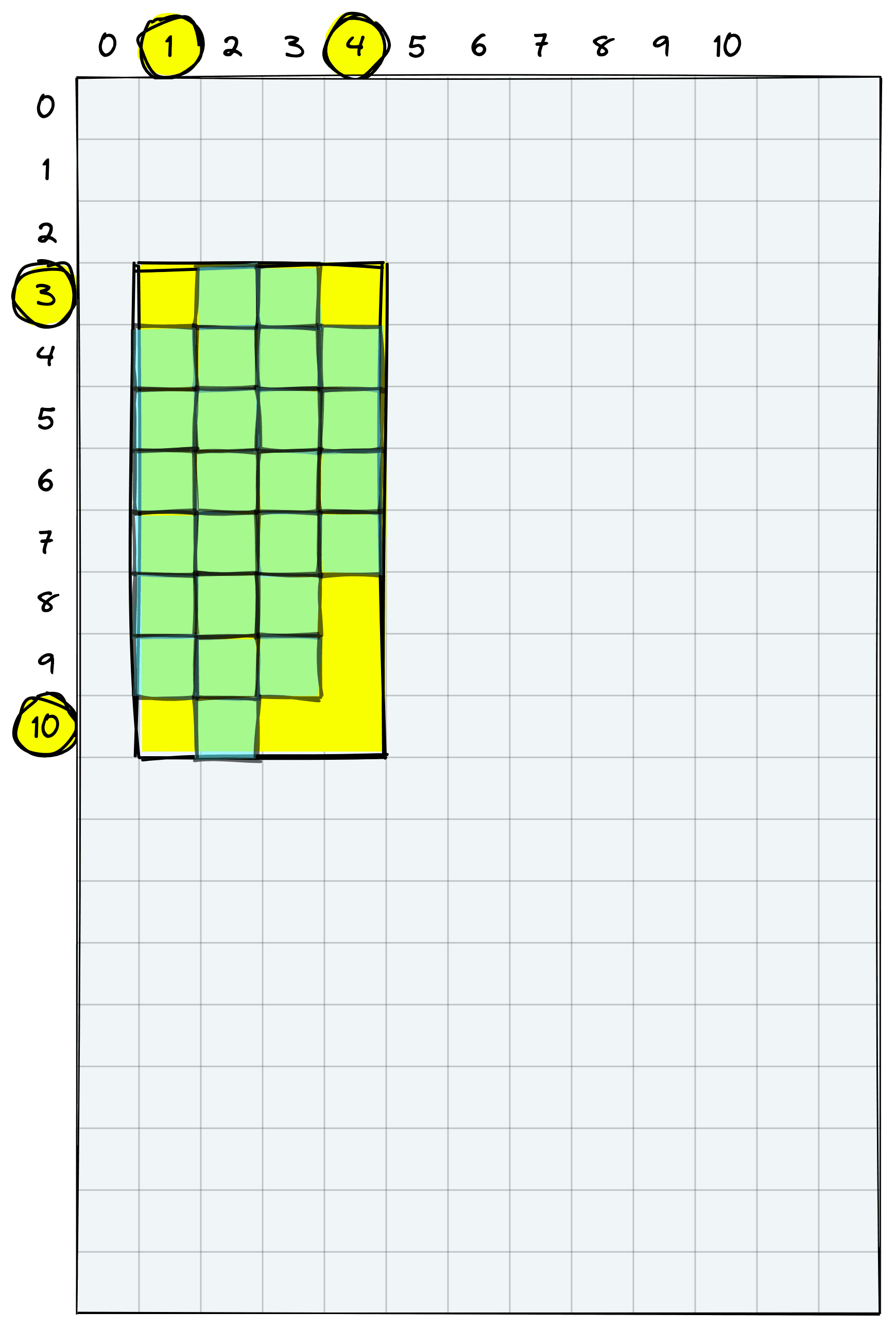
detection = scores > 0.5We can now detect the non-zero positions with the np.nonzero function. The output values represent the x,y coordinates of patches with scores > 0.5.
# non-zero positions
np.nonzero(detection)tensor([[ 3, 2],
[ 3, 3],
[ 4, 1],
[ 4, 2],
[ 4, 3],
[ 4, 4],
[ 5, 1],
[ 5, 2],
[ 5, 3],
[ 5, 4],
[ 6, 1],
[ 6, 2],
[ 6, 3],
[ 6, 4],
[ 7, 1],
[ 7, 2],
[ 7, 3],
[ 7, 4],
[ 8, 1],
[ 8, 2],
[ 8, 3],
[ 9, 1],
[ 9, 2],
[ 9, 3],
[10, 2]])The first column represents the x-coordinates of non-zero positions, and the second column represents the respective y-coordinates.
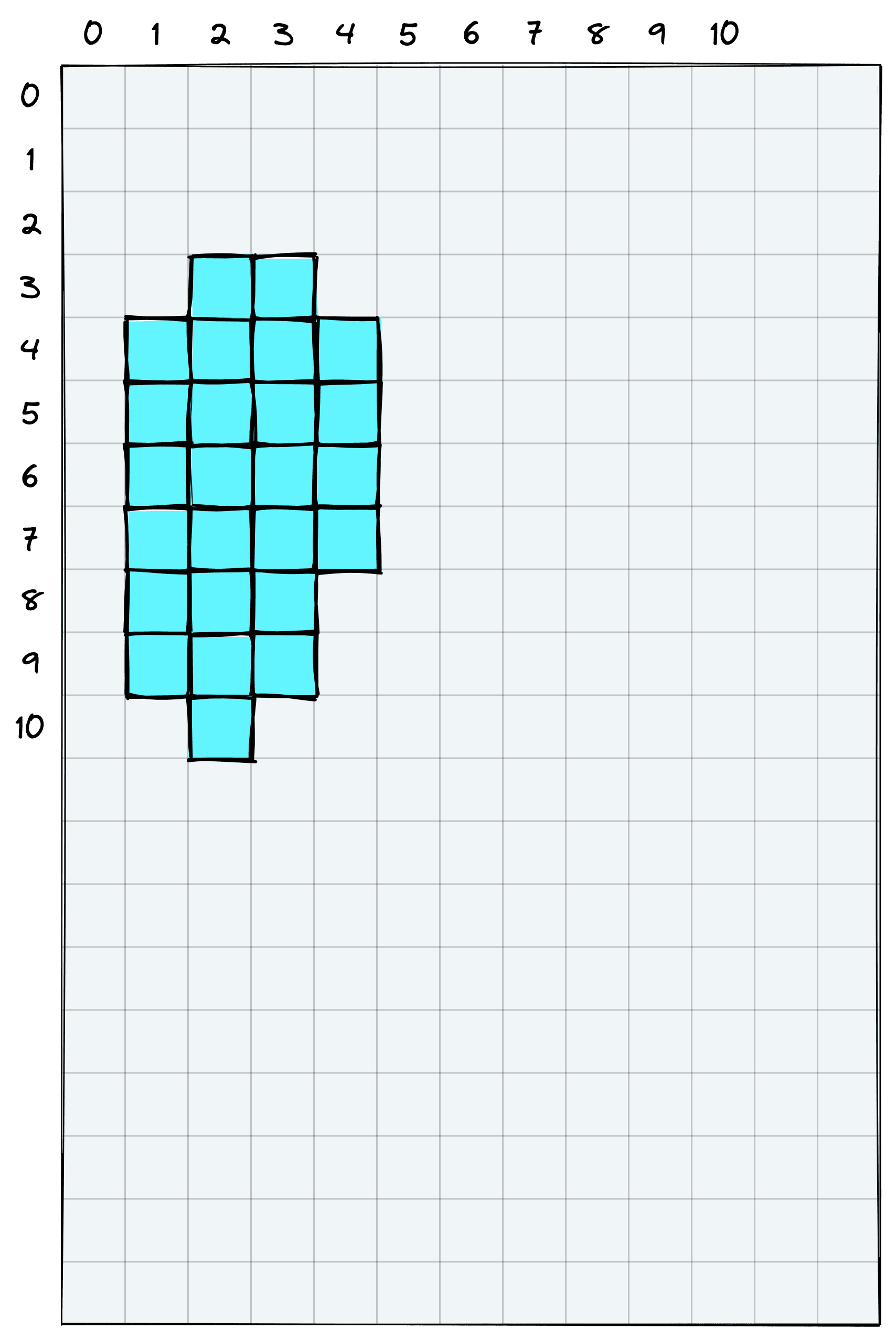
Our bounding box will take each of the edges produced by these non-zero coordinates.
We need the minimum and maximum x and y coordinates to find the box corners.
y_min, y_max = (
    np.nonzero(detection)[:,0].min().item(),
    np.nonzero(detection)[:,0].max().item()+1
)
y_min, y_max(3, 11)x_min, x_max = (
np.nonzero(detection)[:,1].min().item(),
np.nonzero(detection)[:,1].max().item()+1
)
x_min, x_max(1, 5)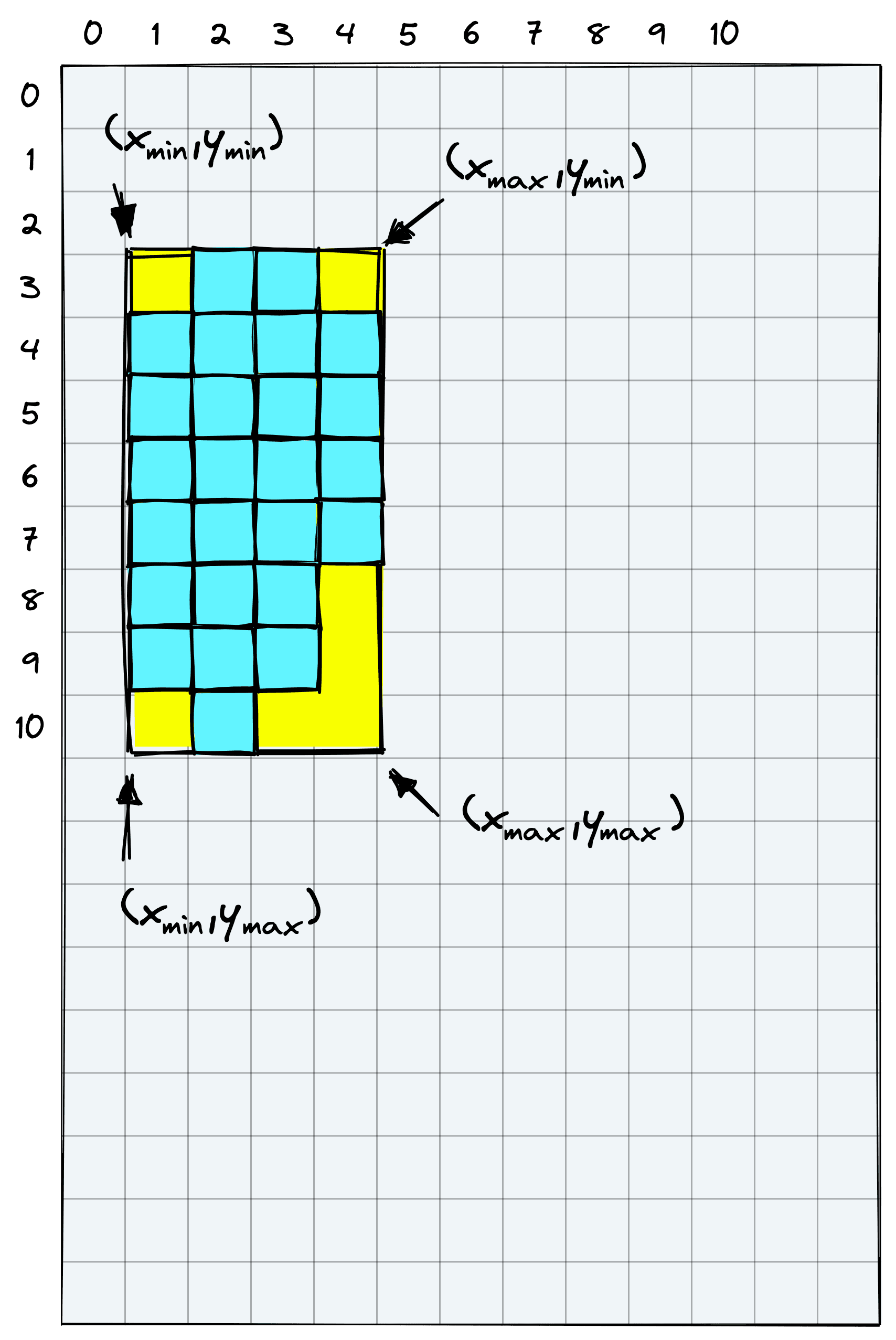
These give us the bounding box coordinates based on patches rather than pixels. To get the pixel coordinates (for the visual), we multiply the coordinates by patch. After that, we calculate the box height and width.
y_min *= patch
y_max *= patch
x_min *= patch
x_max *= patch
x_min, y_min(256, 768)height = y_max - y_min
width = x_max - x_min
height, width(2048, 1024)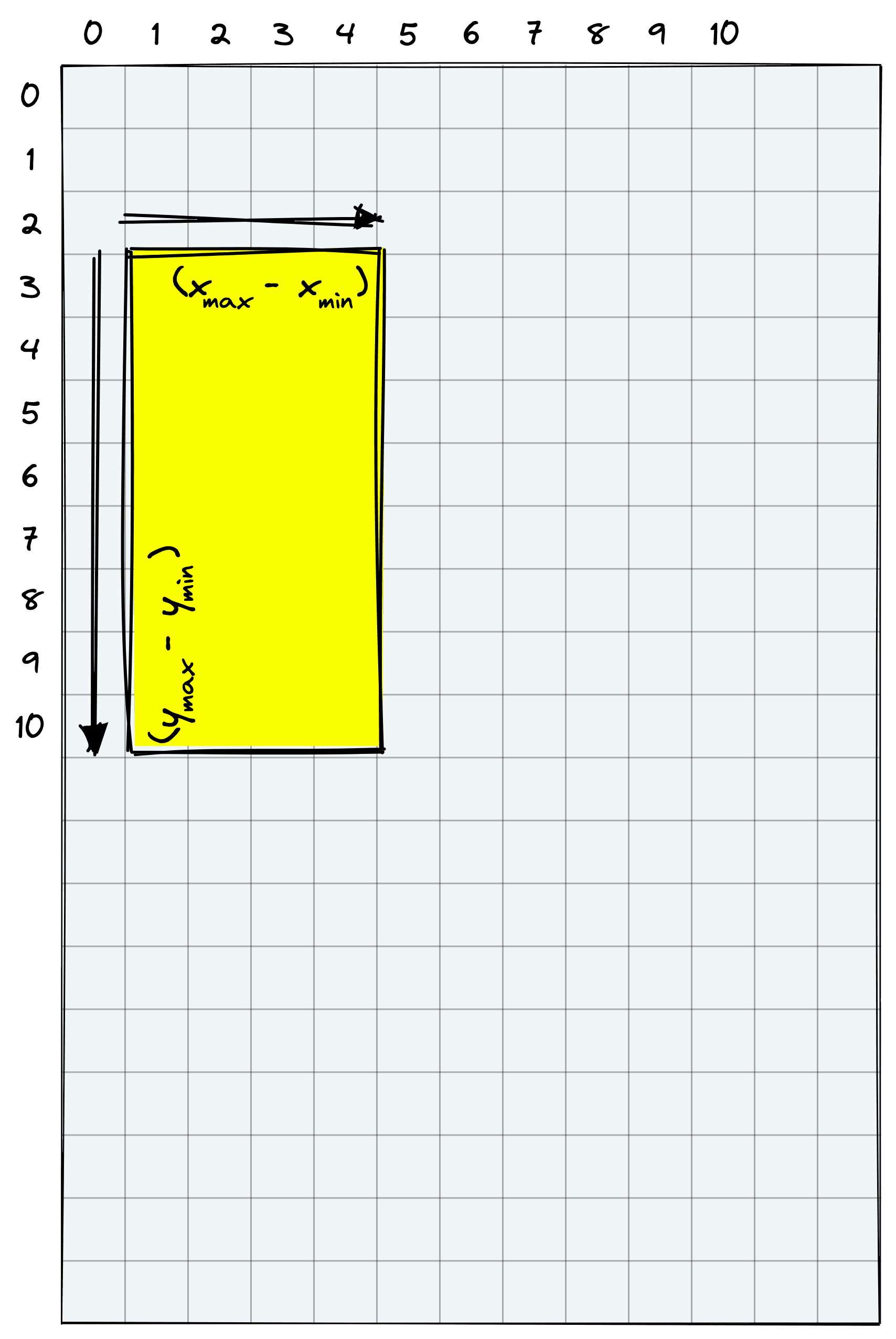
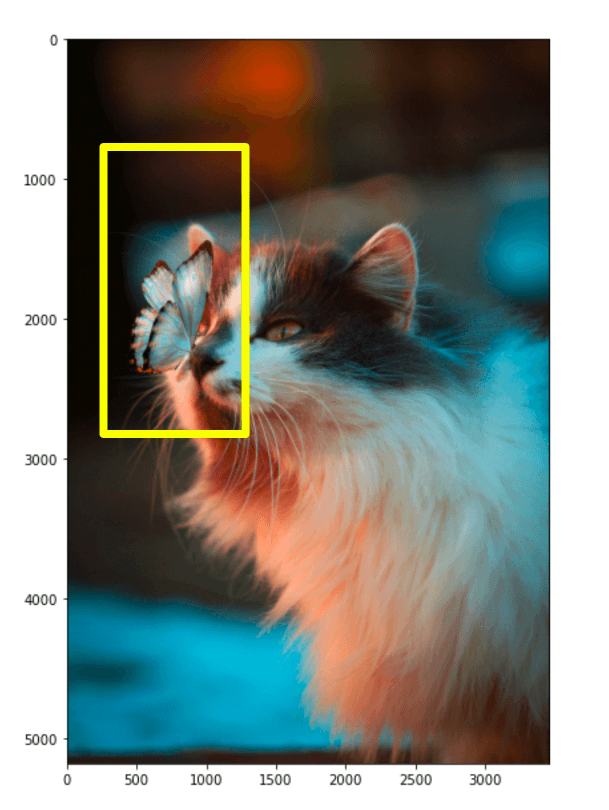
With the x_min, y_min, width, and height values we can use matplotlib.patches to create the bounding box. Before we do that, we convert the original PIL image into a matplotlib-friendly format.
# image shape
img.data.numpy().shape(3, 5184, 3456)# move color channel to final dim
image = np.moveaxis(img.data.numpy(), 0, -1)
image.shape(5184, 3456, 3)Now we visualize everything together:
import matplotlib.patches as patches

fig, ax = plt.subplots(figsize=(Y*0.5, X*0.5))

ax.imshow(image)

# Create a Rectangle patch
rect = patches.Rectangle(
    (x_min, y_min), width, height,
    linewidth=3, edgecolor='#FAFF00', facecolor='none'
)

# Add the patch to the Axes
ax.add_patch(rect)

plt.show()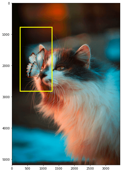
There we have our bounding box visual.
Object Detection
We finally have everything we need to perform object detection for multiple object classes within the same image. The logic is a loop over what we have already built, and we can package it into a neater function like so:
def detect(prompts, img, patch_size=256, window=6, stride=1, threshold=0.5):
    # build image patches for detection
    img_patches = get_patches(img, patch_size)
    # convert image to format for displaying with matplotlib
    image = np.moveaxis(img.data.numpy(), 0, -1)
    # initialize plot to display image + bounding boxes
    fig, ax = plt.subplots(figsize=(Y*0.5, X*0.5))
    ax.imshow(image)
    # process image through object detection steps
    for i, prompt in enumerate(tqdm(prompts)):
        scores = get_scores(img_patches, prompt, window, stride)
        x, y, width, height = get_box(scores, patch_size, threshold)
        # create the bounding box
        rect = patches.Rectangle((x, y), width, height, linewidth=3, edgecolor=colors[i], facecolor='none')
        # add the patch to the Axes
        ax.add_patch(rect)
    plt.show()
(Find the full code here)
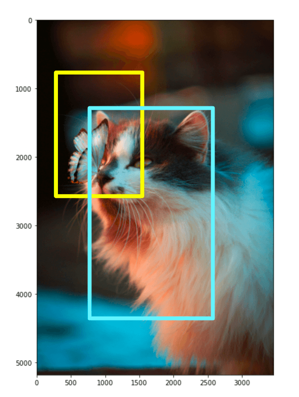
Now we pass a list of class labels and the image to detect. The function will return our image with each detected object annotated with a bounding box.
detect(["a cat", "a butterfly"], img, window=4, stride=1)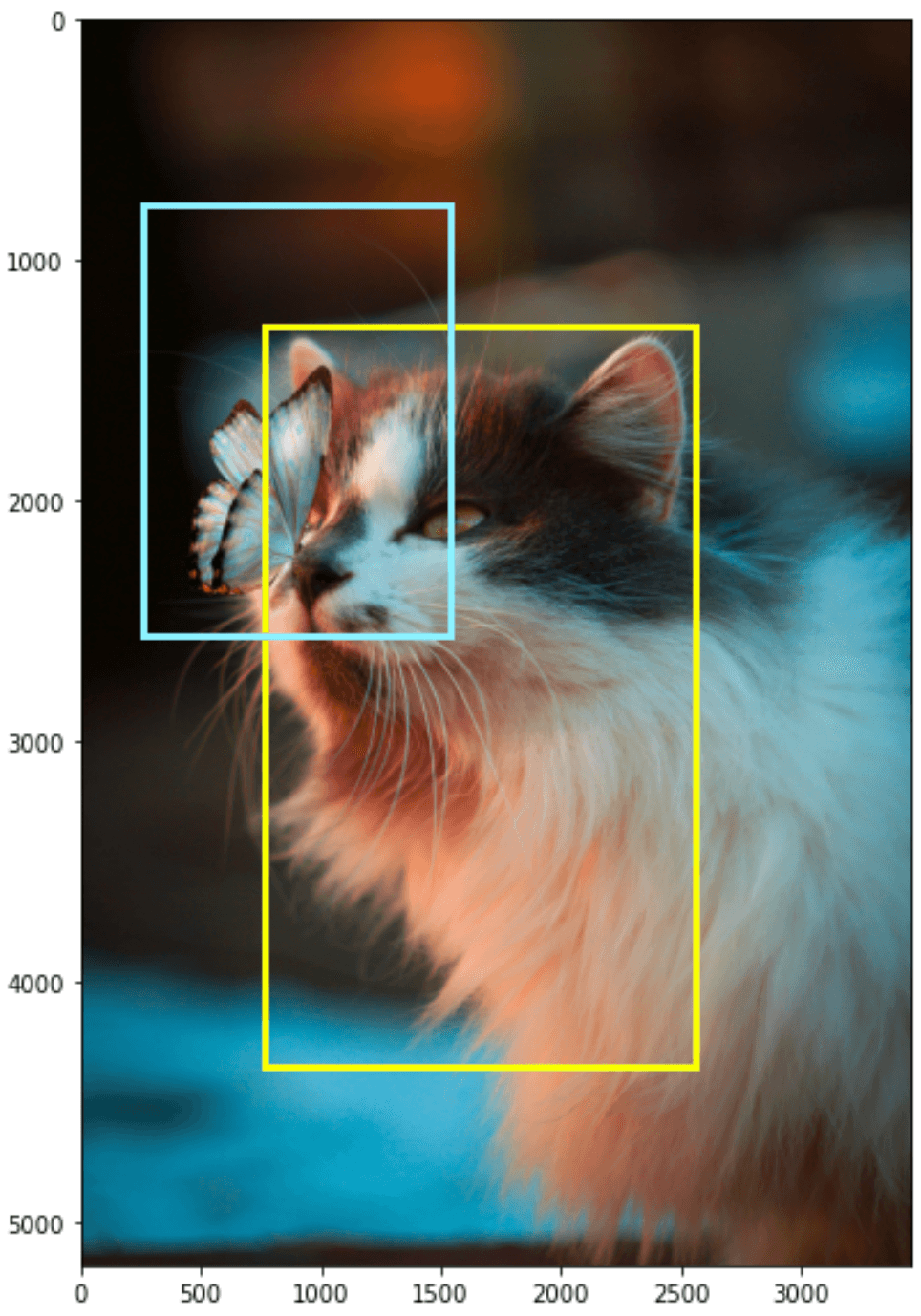
The current implementation is limited to displaying a single object from each class, but this can be solved with a small amount of additional logic.
That’s it for this walkthrough of zero-shot object localization and detection with OpenAI’s CLIP. Zero-shot opens the doors to many organizations and domains that could not perform good object detection due to a lack of training data or compute resources — which is the case for the vast majority of companies.
Multi-modality and CLIP are just part of a trend towards more broadly applicable ML with a much lower barrier to entry. Zero-to-few-shot learning unlocks those previously inaccessible projects and presents us with what will undoubtedly be a giant leap forward in ML capability and adoption across the globe.
Resources
[1] O. Russakovsky et al., ImageNet Large Scale Visual Recognition Challenge (2014)
[2] A. Krizhevsky et al., ImageNet Classification with Deep Convolutional Neural Networks (2012), NeurIPS
[3] A. Radford, J. Kim, et al., Learning Transferable Visual Models From Natural Language Supervision (2021)
[4] F. Bianchi, Domain-Specific Multi-Modal Machine Learning with CLIP (2022), Pinecone Workshop
[5] R. Pisoni, Searching Across Images and Text: Intro to OpenAI’s CLIP (2022), Pinecone Workshop
Was this article helpful?