The components and complexities of time series, and how vectorization can deal with them.
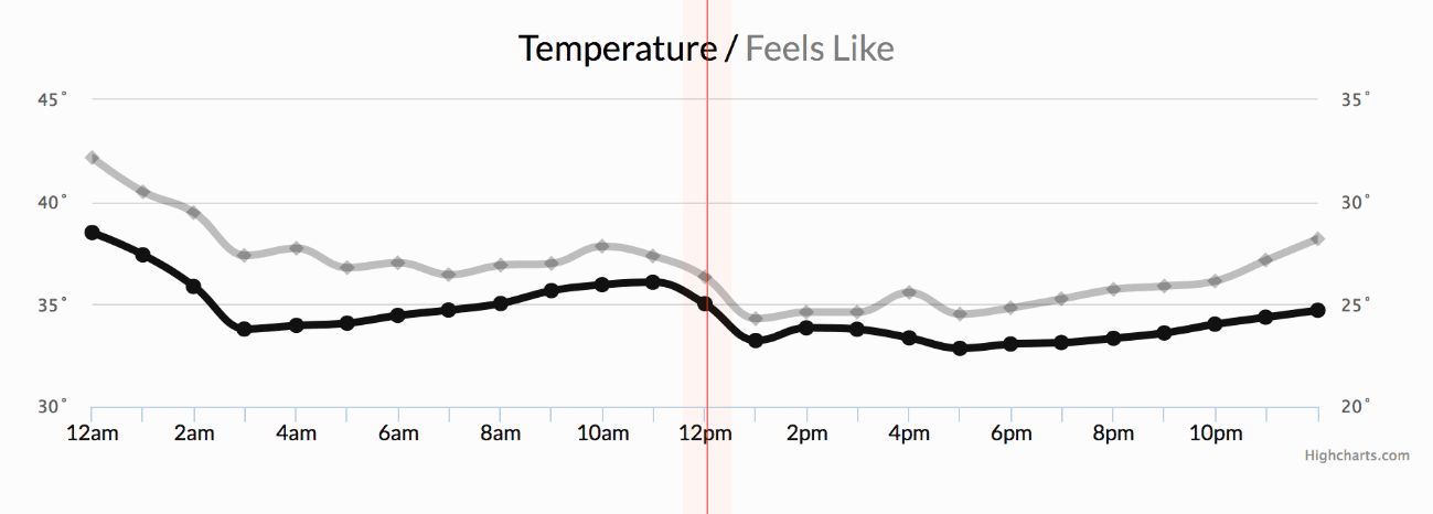
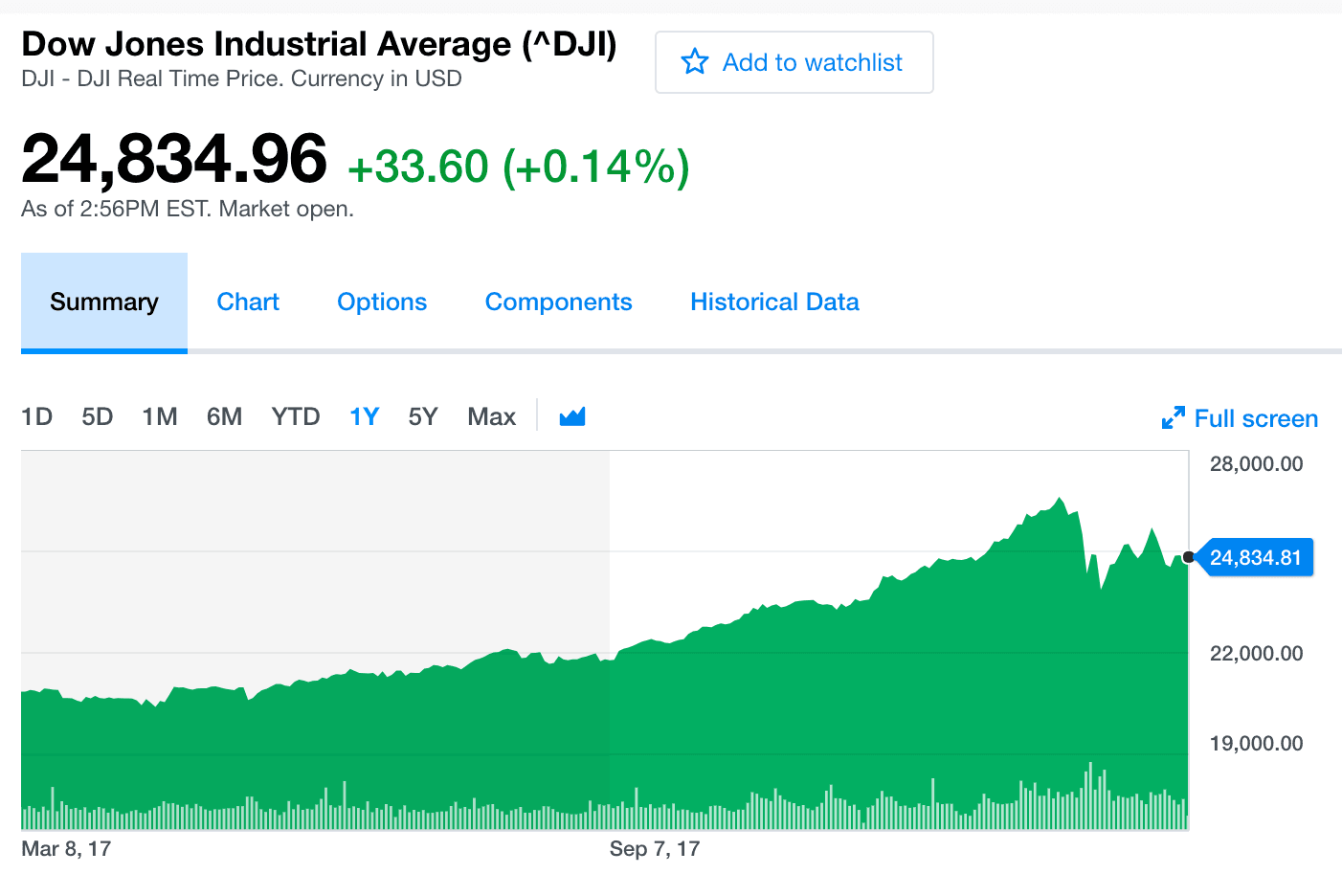
Time series data is all around us. The daily closing price of JP Morgan’s stock, the monthly sales of your company, the annual GDP value of Spain, or the daily maximum temperature values in a given region, are all examples of times series.
A time series is a sequence of observations of data points measured over a time interval. The concept is not new, but we are witnessing an explosion of this type of data as the world gets increasingly measured. Today, sensors and systems are continuously growing the universe of time series datasets. From wearables to cell phones and self-driving cars, the number of connected devices worldwide is set to hit 46 billion.
Depending on the frequency of observations, a time series may typically be hourly, daily, weekly, monthly, quarterly or annual — the data is in order, with a fixed time difference between the occurrence of successive data points.
The concept and applications of time series have become so important, that several tech giants had taken the lead by developing state of the art solutions to ingest, process and analyse them like never before:
- Prophet is open-source software released by Facebook’s Core Data Science team. It’s used in many applications across Facebook for producing reliable forecasts for planning and goal setting, and it includes many possibilities for users to tweak and adjust forecasts. The solution is robust to outliers, missing data, and dramatic changes in the time series.
- Amazon Forecast is a fully managed service that uses Machine Learning to deliver highly accurate forecasts based on the same technology that powers Amazon.com. It builds precise forecasts for virtually any business condition, including cash flow projections, product demand and sales, infrastructure requirements, energy needs, and staffing levels.
- Uber’s Forecasting Platform team created Omphalos, which is a time series back testing framework that generates efficient and accurate comparisons of forecasting models across languages and streamlines the model development process, thereby improving the customer experience.
- SAP Analytics Cloud offers an automatic time series forecasting solution to perform advanced statistical analysis and generate forecasts by analyzing trends, fluctuations and seasonality. The algorithm works by analyzing the historical data to identify the existing patterns in the data and then using those patterns, projects the future values.
Time Series is Different
The “time component” in a time series provides an internal structure that must be accounted for, which makes it very different to any other data type, and sometimes more difficult to handle than traditional datasets.
This is the main difference with sequential data, where the order of the data matters, but the timestamp is irrelevant or doesn’t matter (as in the case of a DNA sequence, where the sequence is important but the concept of time is irrelevant).
This means that, unlike other Machine Learning challenges, you can’t just plug in an algorithm at a time series dataset and expect to have a proper result. Time series data can be transformed into supervised learning problems, but the key step is to consider their temporal structure like trends, seasonality, and forecast horizon.
Since there are so many prediction problems that involve time series, first we need to understand their main components.
Anatomy of Time Series
Unlike other data types, time series have a strong identity on their own. This means that we can’t use the usual strategies to analyze and predict them, since traditional analytical tools fail at capturing their temporal component.
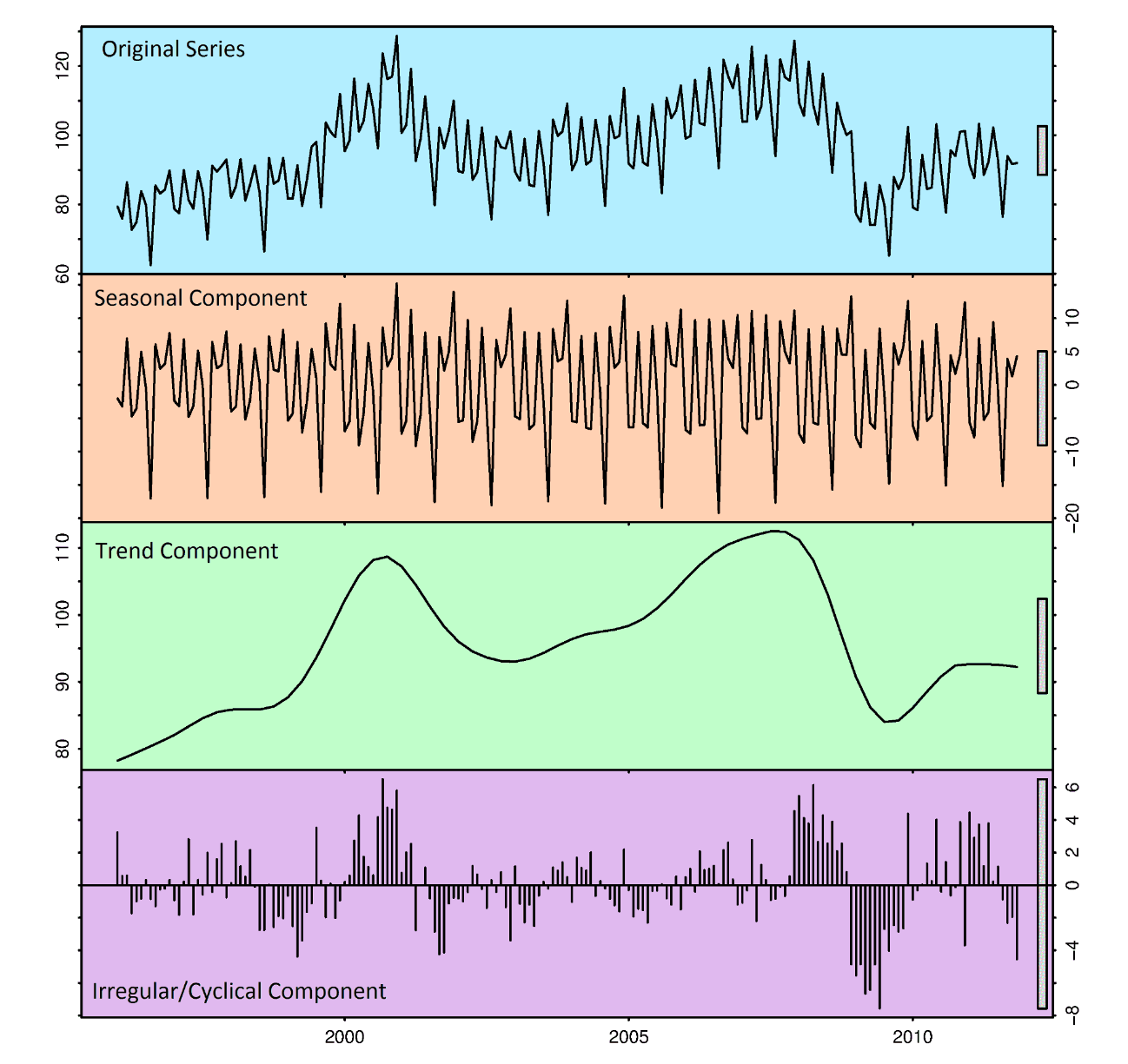
A good way to get a feel of how a time series pattern behaves is to break the time series into its many distinct components. The decomposition of a time series is a task that deconstructs a time series into several pieces, each representing one of the underlying categories of the pattern. Time series decomposition is built on the assumption that data arises as the result of the combination of some underlying components:
- Base Level: This represents the average value in the series.
- Trend: is observed when there is a sustained increasing or decreasing slope observed in the time series.
- Seasonality: Occurs when there is a distinct repeated pattern observed between regular intervals due to seasonal factors, whether it is the month of the year, the day of the month, weekdays, or even times of the day. For example, retail stores sales will be high during weekends and festival seasons.
- Error: The random variation in the series.
All series have a base level and error, while the trend and seasonality may or may not exist. This way, a time series may be imagined as a combination of the base level, trend, seasonality, and error terms.
Another aspect to consider is cyclic behavior. This happens when the rise and fall pattern in the series does not happen in fixed calendar-based intervals, like increases in retail sales that occur around December in response to Christmas or increases in water consumption in summer due to warmer weather.
Care should be taken to not confuse the ‘cyclic’ effect with the ‘seasonal’ effect. So, how to differentiate between a ‘cyclic’ vs ‘seasonal’ pattern?
If patterns are not of fixed calendar-based frequencies, then it is cyclic. Because, unlike seasonality, cyclic effects are typically influenced by the business and other socio-economic factors.
Forecasting
What if besides analyzing a time series, we could predict it? Forecasting is the process of predicting future behaviors based on current and past data.
A time series represents the relationship between two variables: time is one of them, and the measured value is the second one. From a statistical point of view, we can think of the value we want to forecast as a “random variable”.
A random variable is a variable that is subject to random variations so it can take on multiple different values, each with an associated probability.
A random variable doesn’t have a specific value, but rather a collection of potential values. After a measurement is taken and the specific value is revealed, then the random variable ceases to be a random variable and becomes data.
The set of values that this random variable could take, along with their relative probabilities, is known as the “probability distribution”. When forecasting, we call this the forecast distribution. This way, when referring to the “forecast,” we usually mean the average value of the forecast distribution.
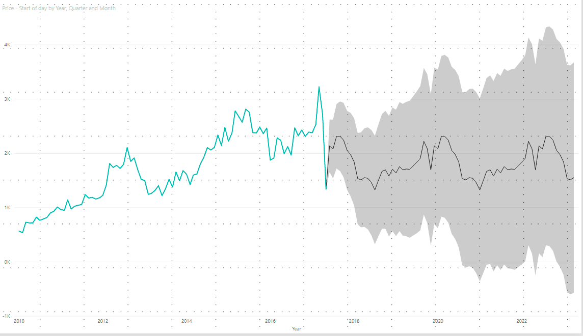
The example on the image above highlights the importance of considering uncertainty. Can we assure how the future will unfold? Of course not, and for this reason it’s important to define prediction intervals (lower and upper boundaries) in which the forecast value is expected to fall.
Statistical time series methods have dominated the forecasting landscape because they are heavily studied and understood, robust, and effective on many problems. Some popular examples of these are ARIMA (autoregressive integrated moving average), Exponential Smoothing methods such as Holt-Winters, and Theta.
However, recent impressive results of Machine Learning methods on time series forecasting tasks triggered a big shift towards these types of models. The year 2018 marked a crucial year when the M4 forecasting competition was won for the first time with a model using Machine Learning techniques. Using this kind of approach, models are able to extract patterns not just from a single time series, but from collections of them. Machine Learning models like Artificial Neural Networks can ingest multiple time series and produce tremendous performances. Nevertheless, these models are “black boxes” that become challenging when interpretability is required.
Decomposing a time series into its different elements allows us to perform unbiased forecasting and brings insights into what might happen in the future. Forecasting is a key activity through different industries and sectors, and those who get it right have a competitive advantage over those who don’t.
By now it becomes clear that we need more than standard techniques to deal with time series. Time series embeddings represent a novel way to uncover insights and perform Machine Learning tasks.
Embeddings to the Rescue
Distance measurement between data examples is a key component of many classification, regression, clustering, and anomaly detection algorithms for time series. For this reason, it’s critical to develop time series representations that can be used to improve the results over these tasks.
Time series embeddings are a representation of time data in the form of vector embeddings that can be used by different models, improving their performance. Vector embeddings are well known and pretty successful in domains like Natural Language Processing and Graphs, but uncommon within time series. Why? Because time series can be challenging to vectorize. Sequential data elude a straightforward definition of similarity because of the necessity of alignment between examples, but time series similarity is also dependent on the task at hand, further complicating the matter.
Fortunately, there are methods that make time-series vectorization a straightforward process. For example, Time2Vec serves as a vector representation for time series that can be used by many models and Artificial Neural Networks architectures like Long Short Term Memory (LSTM), which excel at time series challenges. Time2Vec can be reproduced and used with Python.
Once your time series are vectorized, you can use Pinecone to store and search for them in an easy-to-use and efficient environment. Check out this example showing how to perform time-series “pattern” matching to find out the most similar stock trends.
Was this article helpful?