Vector search powers some of the most popular services in the world. It serves your Google results, delivers the best podcasts on Spotify, and accounts for at least 35% of consumer purchases on Amazon [1][2].
In this article, we will use vector search applied to language, called semantic search, to build a GIF search engine. Unlike more traditional search where we rely on keyword matching, semantic search enables search based on the human meaning behind text and images. That means we can find highly relevant GIFs with natural language prompts.
Preview of the GIF search app available here.
The pipeline for a project like this is simple, yet powerful. It can easily be adapted to tasks as diverse as video search or answering Super Bowl questions, or as we’ll see, finding GIFs.
All supporting notebooks and scripts can be found here.
GIF Dataset
We will be using the TGIF dataset found on GitHub here. To get the dataset we can use wget (alternatively, download it manually), and unzip.
wget https://github.com/raingo/TGIF-Release/archive/master.zip

unzip master.zip
In these unzipped files we should be able to find a file named tgif-v1.0.tsv inside the data directory. We’ll use pandas to load the file using \t as the field delimiter.
import pandas as pd

# Load dataset to a pandas dataframe
df = pd.read_csv(
    "./TGIF-Release-master/data/tgif-v1.0.tsv",
    delimiter="\t",
    names=['url', 'description']
)
df.head() url \
0 https://38.media.tumblr.com/9f6c25cc350f12aa74...
1 https://38.media.tumblr.com/9ead028ef62004ef6a...
2 https://38.media.tumblr.com/9f43dc410be85b1159...
3 https://38.media.tumblr.com/9f659499c8754e40cf...
4 https://38.media.tumblr.com/9ed1c99afa7d714118...
description
0 a man is glaring, and someone with sunglasses ...
1 a cat tries to catch a mouse on a tablet
2 a man dressed in red is dancing.
3 an animal comes close to another in the jungle
4 a man in a hat adjusts his tie and makes a wei... The dataset contains GIF URLs and their descriptions in natural language. We can take a look at the first five GIFs.
for _, gif in df[:5].iterrows():
  HTML(f"<img src={gif['url']} style='width:120px; height:90px'>")
print(gif["description"])<IPython.core.display.HTML object>a man is glaring, and someone with sunglasses appears.
<IPython.core.display.HTML object>a cat tries to catch a mouse on a tablet
<IPython.core.display.HTML object>a man dressed in red is dancing.
<IPython.core.display.HTML object>an animal comes close to another in the jungle
<IPython.core.display.HTML object>a man in a hat adjusts his tie and makes a weird face.
We will find that there are some duplicate URLs, but these do not necessarily indicate duplicate records as a single GIF can be assigned multiple descriptions.
dupes = df['url'].value_counts().sort_values(ascending=False)
dupes.head()https://38.media.tumblr.com/ddbfe51aff57fd8446f49546bc027bd7/tumblr_nowv0v6oWj1uwbrato1_500.gif 4
https://33.media.tumblr.com/46c873a60bb8bd97bdc253b826d1d7a1/tumblr_nh7vnlXEvL1u6fg3no1_500.gif 4
https://38.media.tumblr.com/b544f3c87cbf26462dc267740bb1c842/tumblr_n98uooxl0K1thiyb6o1_250.gif 4
https://33.media.tumblr.com/88235b43b48e9823eeb3e7890f3d46ef/tumblr_nkg5leY4e21sof15vo1_500.gif 4
https://31.media.tumblr.com/69bca8520e1f03b4148dde2ac78469ec/tumblr_npvi0kW4OD1urqm0mo1_400.gif 4
Name: url, dtype: int64dupe_url = "https://33.media.tumblr.com/88235b43b48e9823eeb3e7890f3d46ef/tumblr_nkg5leY4e21sof15vo1_500.gif"
dupe_df = df[df['url'] == dupe_url]
# let's take a look at this GIF and it's duplicated descriptions
for _, gif in dupe_df.iterrows():
HTML(f"<img src={gif['url']} style='width:120px; height:90px'>")
print(gif["description"])<IPython.core.display.HTML object>two girls are singing music pop in a concert
<IPython.core.display.HTML object>a woman sings sang girl on a stage singing
<IPython.core.display.HTML object>two girls on a stage sing into microphones.
<IPython.core.display.HTML object>two girls dressed in black are singing.
With our data, we can move on to building the search pipeline.
Search
The search pipeline will at a high level take our natural language query like “a dog talking on the phone” and search through the existing GIF descriptions for anything that has a similar meaning to this query.
In this context, we describe meaning as semantic similarity, both of which are loaded terms and could refer to many things. For example, are the two phrases "the dog eats lunch" and "the dog does not eat lunch" similar? In this case, it would depend very much on our use case.
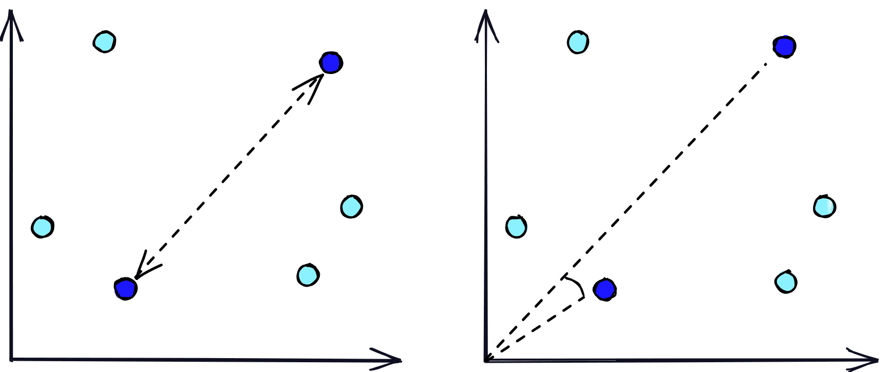
Another example: which of the following two sentences are the most similar?
A: the stock market took a turn for the worse B: how did the stock market do today? C: the stock market performed worse than expected
If we wanted to find phrases with similar meaning then the obvious choice would be A and C. Matching those with B would make little sense. However, this is not the case if we are searching for similar question-answer pairs; in that case, B should match very closely with A and C.
It’s important to identify what your use case requires in it’s definition of “semantic similarity”. For us, we really want to identify generic similarity. That is, we want A and C to match, and B to not match either of those.
To do this, we will transform our phrases into dense vector embeddings. These dense vectors can be stored in a vector database where we can very quickly compare vectors and identify those that are most similar based on metrics like Euclidean distance and cosine similarity.
The vector database handles the storage and fast search of our vector embeddings, but we still need a way to create these embeddings. To do that we use NLP transformer models called retrievers that are fine-tuned for creating sentence embeddings. These sentence embeddings/vectors are able to numerically represent the meaning behind the text that they represent.
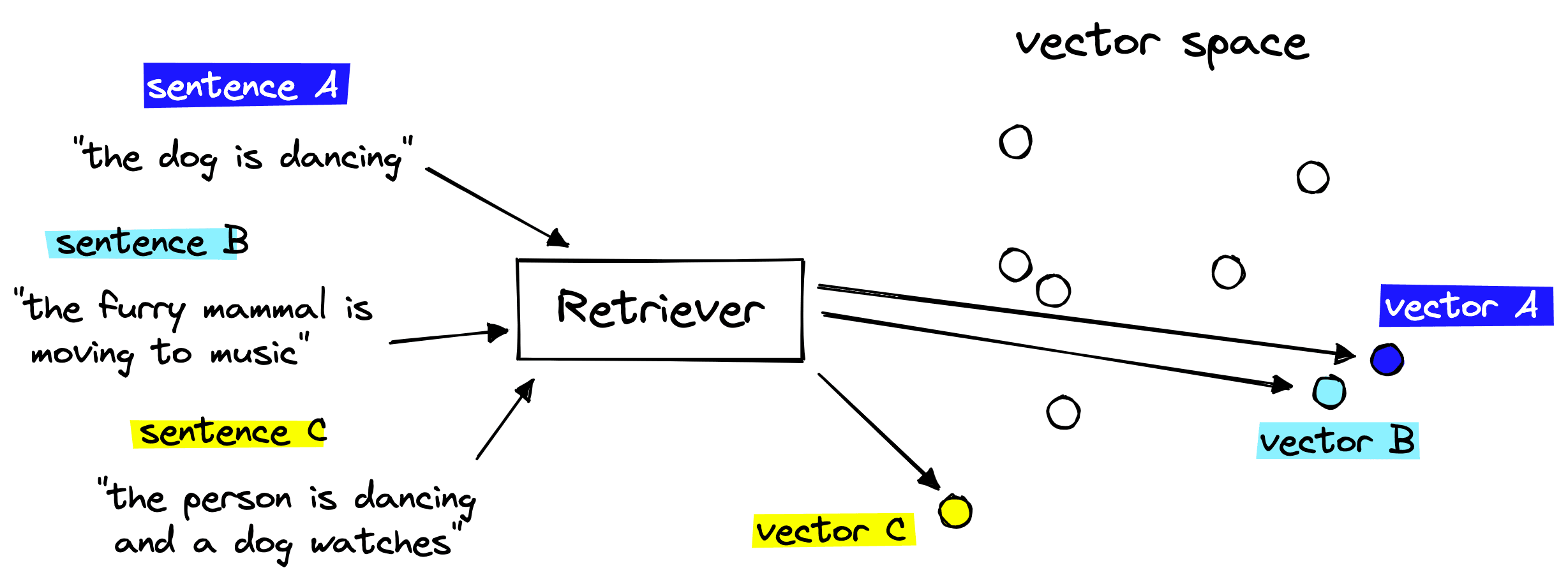
Putting these two components together gives us a semantic search pipeline that we can use to retrieve semantically similar GIF descriptions given a query.
GIF search pipeline covering the one-time indexing step (left) and querying (right).
Let’s take a look at how we can put all of this together.
Initializing Components
We will start by initializing our retriever model. Many of the most powerful retrievers use a sentence transformer architecture, which are best supported via the sentence-transformers library, installed via a pip install sentence-transformers.
To find sentence transformer models we go to huggingface.co/models and search for sentence-transformers for the official sentence transformer models. However, there are other models we can use like the all-MiniLM-L6-v2 sentence transformer trained during a special event on over 1B training pairs. We will use this model.
from sentence_transformers import SentenceTransformer

# Initialize retriever with SentenceTransformer model
retriever = SentenceTransformer('sentence-transformers/all-MiniLM-L6-v2')
retrieverSentenceTransformer(
(0): Transformer({'max_seq_length': 256, 'do_lower_case': False}) with Transformer model: BertModel
(1): Pooling({'word_embedding_dimension': 384, 'pooling_mode_cls_token': False, 'pooling_mode_mean_tokens': True, 'pooling_mode_max_tokens': False, 'pooling_mode_mean_sqrt_len_tokens': False})
(2): Normalize()
)There are a couple of important details here:
max_sequence_length=128means the model can read up to 128 input tokens.word_embedding_size=384actually refers to the sentence embedding size. This means the model will output a 384-dimensional vector representation of the input text.
For the short several-word GIF descriptions of our dataset a maximum sequence length of 128 is more than enough.
We need to use the sentence embedding size when initializing our vector database, so we store that in the embed_dim variable above.
To initialize our vector database we first need to sign up for a free Pinecone API key and install the Pinecone Python client via pip install pinecone-client. Once ready, we initialize:
import pinecone

# Connect to pinecone environment
pinecone.init(
    api_key="YOUR_API_KEY",
    environment="YOUR_ENV"  # find next to API key
)

index_name = 'gif-search'

# check if the gif-search exists
if index_name not in pinecone.list_indexes():
    # create the index if it does not exist
    pinecone.create_index(
        index_name,
        dimension=384,
        metric="cosine"
    )

# Connect to gif-search index we created
index = pinecone.Index(index_name)
Here, we are specifying an index name of 'gif-search'; feel free to choose anything you like. It is simply a name. The metric is more important and depends on the model being used. For our chosen model we can see in its model card that it has been trained to use cosine similarity, hence why we have specified metric='cosine'. Alternative metrics include euclidean and dotproduct.
We’ve initialized both our vector database and retriever components, so we can move on to embedding and indexing our data.
Indexing
The embedding and indexing process is much faster when we perform these steps for multiple records in parallel. However, we cannot process all of our records at once as the retriever model must shift everything it is embedding into on-chip memory, which is limited.
To avoid this limit, while keeping indexing times as fast as possible, we process everything in batches of 64.
from tqdm.auto import tqdm

# we will use batches of 64
batch_size = 64

for i in tqdm(range(0, len(df), batch_size)):
    # find end of batch
    i_end = min(i+batch_size, len(df))
    # extract batch
    batch = df.iloc[i:i_end]
    # generate embeddings for batch
    emb = retriever.encode(batch['description'].tolist()).tolist()
    # get metadata
    meta = batch.to_dict(orient='records')
    # create IDs
    ids = [f"{idx}" for idx in range(i, i_end)]
    # add all to upsert list
    to_upsert = list(zip(ids, emb, meta))
    # upsert/insert these records to pinecone
    _ = index.upsert(vectors=to_upsert)


# check that we have all vectors in index
index.describe_index_stats() 0%| | 0/1966 [00:00<?, ?it/s]{'dimension': 384,
'index_fullness': 0.05,
'namespaces': {'': {'vector_count': 125782}}}Here we are extracting the batch from our data df. We encode the descriptions via our retriever model, create metadata (covering both descriptions and url), and create some string format IDs. From this we have everything we need to create documents, which will look like this:
(
       "some-id-value",
   [0.1, 0.2, 0.1, 0.4 ...],
   {
       'description': "something descriptive",
       'url': "https://xyz.com"
   }
)
When we upsert these documents to the Pinecone index, we do so in batches of 64. After all of this, we use index.describe_index_stats() to check that we have inserted all 125,782 documents, which we have.
Querying
The final step of querying our data covers:
- Encoding a query like “dogs talking on the phone” to create a query vector,
- Retrieval of similar context vectors from Pinecone,
- Getting relevant GIFs from the URLs found in our metadata fields.
Steps one and two will be performed by a function named search_gif:
def search_gif(query):
    # Generate embeddings for the query
    xq = retriever.encode(query).tolist()
    # Compute cosine similarity between query and embeddings vectors and return top 10 URls
    xc = index.query(xq, top_k=10,
                    include_metadata=True)
    result = []
    for context in xc['matches']:
        url = context['metadata']['url']
        result.append(url)
    return result
To display the GIFs we display HTML <img> elements using the metadata URLs to point to the correct GIFs. We do this using the display_gif function:
def display_gif(urls):
    figures = []
    for url in urls:
        figures.append(f'''
            <figure style="margin: 5px !important;">
              <img src="{url}" style="width: 120px; height: 90px" >
            </figure>
        ''')
    return HTML(data=f'''
        <div style="display: flex; flex-flow: row wrap; text-align: center;">
        {''.join(figures)}
        </div>
    ''')
Let’s test some queries.
gifs = search_gif("a dog being confused")
display_gif(gifs)<IPython.core.display.HTML object>gifs = search_gif("animals being cute")
display_gif(gifs)<IPython.core.display.HTML object>gifs = search_gif("a fluffy dog being cute and dancing like a person")
display_gif(gifs)<IPython.core.display.HTML object>That looks pretty accurate so we’ve managed to put this GIF search pipeline together very easily. With a little added effort we can translate these steps in creating a web app using something like Streamlit.
We’ve successfully built a GIF search tool using a simple semantic search pipeline with out-of-the-box models and Pinecone. This same pipeline can be applied across a variety of domains with very little tweaking.
The ease-of-use and potential of both vector and semantic search have led to a lot of research and applications of both technologies beyond the world of big tech. If you’re interested in seeing other applications of this technology, or would like to share your own, considering joining the Pinecone community.
Resources
[1] M. Osborne, How Retail Brands Can Compete And Win Using Amazon’s Tactics (2017), Forbes
[2] L. Hardesty, The history of Amazon’s recommendation algorithm (2019), Amazon Science
Was this article helpful?