Sparse V3: how Pinecone's sparse index learned to skip



TLDR: Pinecone's V2 sparse index organized posting data in document-major blocks, which forced every query to load the entire index regardless of which terms it contained. V3 reorganizes the index around terms: each term owns its own sequence of posting blocks, and a query only loads the blocks for terms it actually references. From disk, this reduces I/O by 151× for SPLADE queries and 1,428× for BM25 queries, with no loss in recall, and measurably better recall for BM25.
Sparse indexes at Pinecone
In March 2025, Pinecone launched sparse-only indexes, bringing keyword and lexical search into the same serverless platform as dense vector retrieval, supporting both BM25 and learned sparse models including SPLADE and Pinecone's own pinecone-sparse-english-v0.
Sparse retrieval is built on inverted indexes, a data structure at the heart of search engines for decades. Each term gets mapped to a posting list: a record of every document containing it and a relevance score for that document. Traditional scoring functions like BM25 weight terms by frequency within a document and rarity across the corpus. Learned sparse models like SPLADE go further, using a transformer to assign context-aware weights and expand a document's representation to include related terms. A document about machine learning might score non-zero on "training" and "inference" even without those words appearing verbatim. Pinecone's implementation runs this on the MaxScore algorithm, which makes retrieval fast at scale by skipping documents that can't beat the current top-k threshold rather than scoring every candidate.
Supporting sparse vectors alongside dense, operating a separate Elasticsearch or Solr cluster is no longer needed, and the search pipeline gets further consolidated. Sparse and dense indexes are queryable together in a single index (sparse for keyword matching, dense for semantic breadth) with Pinecone managing both.
The scale problem
The architecture that powered V1 and V2 organized posting data in what's called a document-major layout. Documents are divided into groups by ordinal position (1–1000, 1001–2000, and so on). Each group gets a block on disk containing the interleaved posting data of all terms in any of the group’s documents.
At query time, the search algorithm has to read each of these blocks, because any block might contain postings for any of the query's terms. A query for "apple" and "orange" reads the block covering documents 1–1000, then 1001–2000, then every other block through the entire index. There's no way to skip ahead without reading.
When an index fits in memory, this is survivable. SIMD scoring is fast, and scanning several gigabytes at memory bandwidth completes in hundreds of milliseconds. But as sparse indexes gained adoption, larger workloads appeared. A billion-vector SPLADE index can run to hundreds of gigabytes. At that size, keeping the full index in memory is expensive. And in a serverless environment where many users share the same underlying hardware, it often isn't feasible: memory is allocated dynamically across workloads, so one large index needing most of the available memory delays other active indexes.
When an index can't stay in memory, every query becomes a series of disk reads— and reads from disk are orders of magnitude slower than memory. The V2 disk benchmarks make this concrete: every SPLADE query took 3,407 milliseconds regardless of what it was searching for, at p50, p90, and p99. The completely flat distribution exposed disk throughput as the limiting factor.
For billion-scale indexes, the only path to sub-second latency used to be dedicated hardware sized to keep the full index in memory.
What V3 changes
We needed a way to reduce disk reads. Specifically, instead of loading the whole index into memory, we needed to devise a method to identify and load only the relevant postings. That way, a query touching 2 terms out of a 50,000-term vocabulary still had to read all 50,000 terms' worth of posting data (because they were packed together indistinguishably).
V3 overhauls the layout so queries can skip directly to what they need.
- Term-major layout: Each term gets its own blocks on disk; a query only loads data for the terms it contains.
- In-memory term directory: A compact map keeps every term's disk location in memory, so finding a term costs no I/O.
- Metadata-first block skipping: A small summary block per term lets the algorithm decide what to skip before loading any posting data.
- Compressed posting blocks: Doc IDs and scores are compressed per-term, reducing block sizes up to x2.5.
Organizing by term instead of by document range
V3 flips the grouping strategy: it groups posting data by term instead of document range. All of "apple"'s postings live in their own contiguous sequence of blocks on disk; all of "orange"'s postings live in another sequence elsewhere. A query then reads only the blocks for the terms it actually contains. A SPLADE query typically includes dozens of non-zero terms; a BM25 query, just a few. Against a vocabulary of tens of thousands, both are a small fraction of the index to load.
A compact directory that lives in memory
Reorganizing around terms creates a new problem: with posting data scattered across potentially tens of thousands of separate locations on disk, how does the search algorithm find a given term's blocks without scanning the index?
V3 solves this with a term directory, a compact map stored in the index metadata that records, for each term, where its posting data begins on disk. The metadata loads into memory when the index is opened and stays there. Every term lookup is an in-memory operation; finding a term's disk location costs no I/O.
The directory uses Elias-Fano encoding, which compresses sorted integer sequences while preserving O(1) lookup. For 100,000 terms, the result fits in about 300 KB (small enough to stay in the CPU’s L2 cache).
| Structure | Size (100K Terms) | Lookup |
|---|---|---|
| Sorted array of pairs | ~800 KB | O(log n) |
| Hash map | ~2.4 MB | O(1) |
| Elias-Fano | ~300 KB | O(1)¹ |
¹ O(1) positional access by term ID; the term dictionary resolves strings to dense integer IDs upstream.
Deciding whether to load a block before loading it
Even after locating a term's posting data, not every block for that term may be worth loading. A term that appears in many documents will have many posting blocks. MaxScore pruning can skip the weaker ones, but applying that logic requires knowing each block's maximum possible score before deciding to load it.
V3 stores this information in a metadata block at the start of each term's data. Before any posting blocks are read, the search algorithm loads this metadata block (a small, fast I/O) and gets back a summary for every posting block the term contains: the range of document IDs in the block, the highest score any posting in the block achieves, and the number of postings. With that summary in hand, three classes of skip decisions happen without reading any posting data: metadata filtering, MaxScore pruning, and position skipping.
Compressing what's left
The blocks that aren't skipped need to be as small as possible to reduce I/O and better fit in the memory cache during scoring. V3 applies two compression techniques that only work best with its term-major layout.
Document ID compression. Rather than storing each document ID as a full 32-bit integer, V3 stores only the offset from the block's minimum document ID. The minimum ID is already recorded in the metadata block, so the decoder knows the reference point before reading any posting data. The maximum offset within a block determines how many bits each offset needs. For example, a block spanning documents 50,000 to 50,128 only needs 7 bits per offset rather than 32. SIMD operations pack and unpack each posting block’s values in a single pass with no branching. The result is 2–2.5× compression for tightly clustered blocks, and meaningful compression even for spread-out ones.
| Block Spread | Bits per ID | Total |
|---|---|---|
| Tight (range < 256) | 8 | 256 B |
| Medium (range < 64K) | 16 | 384 B |
| Wide(range < 1M) | 20 | 448 B |
A full posting block fits in a handful of L1 CPU cache lines.
Per-term score quantization. Scores are stored as single bytes mapped to a score range. Whereas V2 used one range across all terms in a document block to represent score, V3 uses each term's own range. This finer mapping explains V3’s increased recall, especially for BM25 models.
Finding the right heuristics
The performance-critical decisions—window sizing, merge strategy, and scoring granularity—depend on hardware cache geometry and posting list density in ways that resist analytical derivation. How these parameters got tuned turned out to be the most unconventional part of the build, and in some ways more interesting than the structural changes it was optimizing.
The approach: property-based tests and recall benchmarks as the fitness function, with Claude driving hundreds of iterations testing algorithmic combinations, and a human reviewing direction and killing runs that were clearly going wrong. When a property test failed or recall dropped, the loop backtracked. When throughput improved with recall holding, the change was retained. The heuristics that shipped (window sizes tuned to L1 cache, adaptive behavior across posting densities) came from this iterative, empirical process. It worked because the test harness was rigorous enough to trust, as a false pass would have been worse than a slow run.
Results
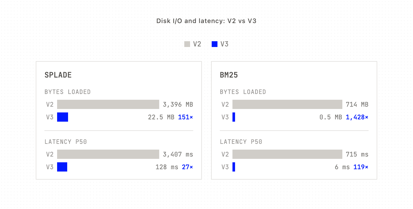
Benchmarks run on MS MARCO, a standard retrieval corpus of 8.8 million documents using SPLADE embeddings (averaging ~45 non-zero query terms) and BM25 (averaging ~3 query terms). BM25 gains are larger because sparse query vectors reference fewer terms, leaving more of the index for V3 to skip.
Scanning under I/O pressure (from disk)
This is the case V3 was built for: an index too large to keep resident, where every query pays in disk reads. Under V2, that meant reading the whole index on every query, no matter how few terms it touched.
| Metric | V2 | V3 | Change |
|---|---|---|---|
| Recall@100 | 1.0000 | 1.0000 | -- |
| Bytes loaded / query (p50) | 3,396 MB | 22.5 MB | 151x less |
| Latency p50 | 3,407 ms | 128 ms | 27x faster |
| Latency p90 | 3,407 ms | 252 ms | 14x faster |
V2's latency is flat across percentiles. Every query did the same work, so every query took the same time (a little over three seconds regardless of what was asked). V3 executes those same queries in a couple hundred milliseconds, scaling by the number of terms involved rather than the flat size of the index.
| Metric | V2 | V3 | Change |
|---|---|---|---|
| Recall@100 | 0.9840 | 0.9840 | -- |
| Bytes loaded / query (p50) | 714 MB | 0.5 MB | 1,428× less |
| Latency p50 | 715 ms | 6 ms | 119× faster |
| Latency p90 | 719 ms | 13 ms | 55× faster |
For a typical short query, V3 reads 1,428× less data and returns in milliseconds, because it pays only for the terms it contains. The recall a user gets back is identical.
The payoff shows up directly in production. One customer running billion-scale sparse queries migrated to V3 and went from multiple seconds per query to 40 milliseconds on the same hardware. For their users, that’s the difference between a search that stalls and one that feels instant. It’s also what makes billion-scale sparse retrieval affordable on shared serverless infrastructure, rather than something that demands dedicated hardware sized to the worst case.
Conclusion
The document-major layout had one flaw that scale exposed: queries couldn't skip all irrelevant data. Every query read the entire index, so a two-term lookup costed as much as scanning everything. This worked well when indices could fit in memory. Once they didn't, every query fell back to disk and the design didn't hold.
V3 reorganizes posting data around terms rather than document ranges:
- each term owns its blocks
- in-memory directory finds them with no I/O
- per-block metadata lets the algorithm skip what it doesn't need before reading it from disk
- per-term compression shrinks what remains
A full-index scan becomes a read that touches only the terms a query contains.
This algorithm runs in all of Pinecone's sparse indexes today (thanks to the compaction process, changing algorithms was a completely online procedure, without disrupting any ongoing operations). Queries pay for what they use, recall holds, and billion-scale sparse retrieval runs on shared serverless infrastructure alongside dense retrieval in a single pipeline.
Was this article helpful?