Rerankers and Two-Stage Retrieval

Retrieval Augmented Generation (RAG) is an overloaded term. It promises the world, but after developing a RAG pipeline, there are many of us left wondering why it doesn't work as well as we had expected.

As with most tools, RAG is easy to use but hard to master. The truth is that there is more to RAG than putting documents into a vector DB and adding an LLM on top. That can work, but it won't always.

This ebook aims to tell you what to do when out-of-the-box RAG doesn't work. In this first chapter, we'll look at what is often the easiest and fastest to implement solution for suboptimal RAG pipelines — we'll be learning about rerankers.

Recall vs. Context Windows

Before jumping into the solution, let's talk about the problem. With RAG, we are performing a semantic search across many text documents — these could be tens of thousands up to tens of billions of documents.

To ensure fast search times at scale, we typically use vector search — that is, we transform our text into vectors, place them all into a vector space, and compare their proximity to a query vector using a similarity metric like cosine similarity.

For vector search to work, we need vectors. These vectors are essentially compressions of the "meaning" behind some text into (typically) 768 or 1536-dimensional vectors. There is some information loss because we're compressing this information into a single vector.

Because of this information loss, we often see that the top three (for example) vector search documents will miss relevant information. Unfortunately, the retrieval may return relevant information below our top_k cutoff.

What do we do if relevant information at a lower position would help our LLM formulate a better response? The easiest approach is to increase the number of documents we're returning (increase top_k) and pass them all to the LLM.

The metric we would measure here is recall — meaning "how many of the relevant documents are we retrieving". Recall does not consider the total number of retrieved documents — so we can hack the metric and get perfect recall by returning everything.

Unfortunately, we cannot return everything. LLMs have limits on how much text we can pass to them — we call this limit the context window. Some LLMs have huge context windows, like Anthropic's Claude, with a context window of 100K tokens [1]. With that, we could fit many tens of pages of text — so could we return many documents (not quite all) and "stuff" the context window to improve recall?

Again, no. We cannot use context stuffing because this reduces the LLM's recall performance — note that this is the LLM recall, which is different from the retrieval recall we have been discussing so far.

When storing information in the middle of a context window, an LLM's ability to recall that information becomes worse than had it not been provided in the first place [2].

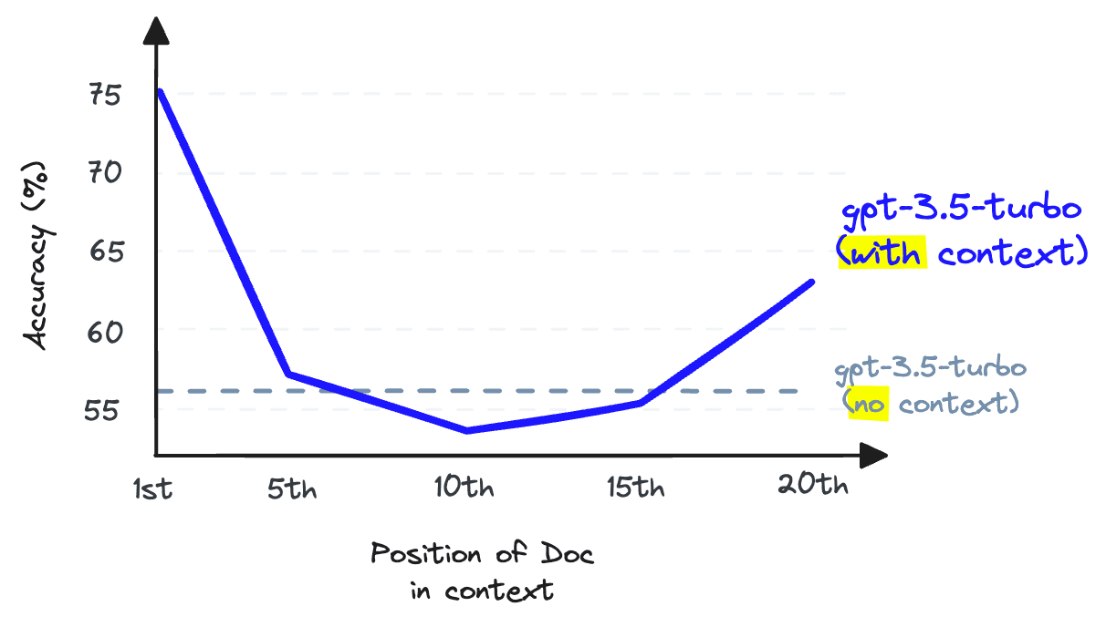
LLM recall refers to the ability of an LLM to find information from the text placed within its context window. Research shows that LLM recall degrades as we put more tokens in the context window [2]. LLMs are also less likely to follow instructions as we stuff the context window — so context stuffing is a bad idea.

We can increase the number of documents returned by our vector DB to increase retrieval recall, but we cannot pass these to our LLM without damaging LLM recall.

The solution to this issue is to maximize retrieval recall by retrieving plenty of documents and then maximize LLM recall by minimizing the number of documents that make it to the LLM. To do that, we reorder retrieved documents and keep just the most relevant for our LLM — to do that, we use reranking.

Power of Rerankers

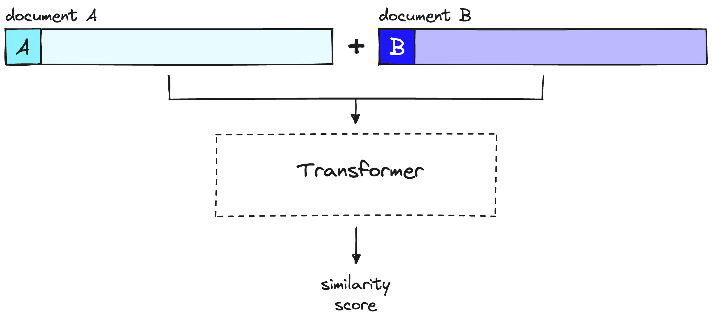
A reranking model — also known as a cross-encoder — is a type of model that, given a query and document pair, will output a similarity score. We use this score to reorder the documents by relevance to our query.

A two-stage retrieval system. The vector DB step will typically include a bi-encoder or sparse embedding model.

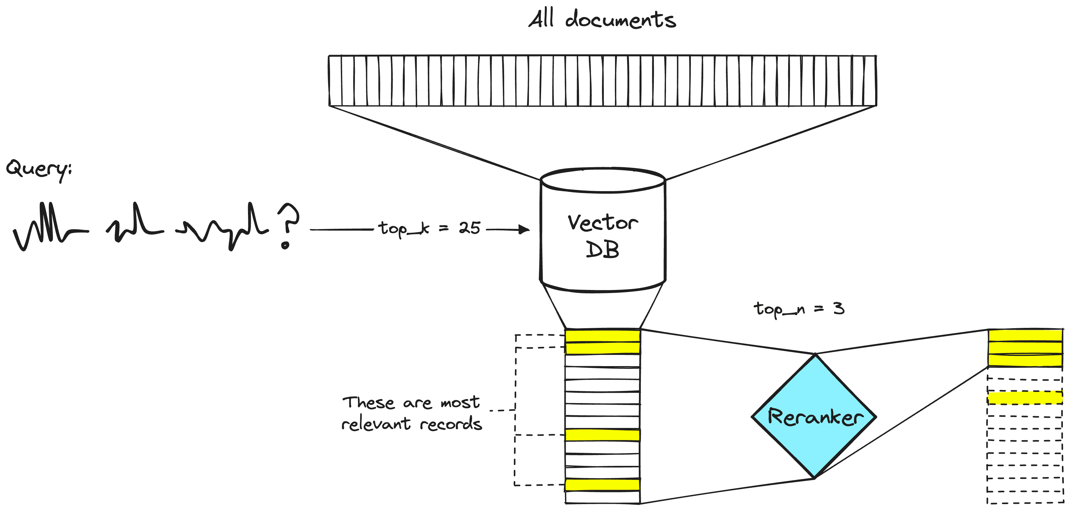
Search engineers have used rerankers in two-stage retrieval systems for a long time. In these two-stage systems, a first-stage model (an embedding model/retriever) retrieves a set of relevant documents from a larger dataset. Then, a second-stage model (the reranker) is used to rerank those documents retrieved by the first-stage model.

We use two stages because retrieving a small set of documents from a large dataset is much faster than reranking a large set of documents — we'll discuss why this is the case soon — but TL;DR, rerankers are slow, and retrievers are fast.

Why Rerankers?

If a reranker is so much slower, why bother using them? The answer is that rerankers are much more accurate than embedding models.

The intuition behind a bi-encoder's inferior accuracy is that bi-encoders must compress all of the possible meanings of a document into a single vector — meaning we lose information. Additionally, bi-encoders have no context on the query because we don't know the query until we receive it (we create embeddings before user query time).

On the other hand, a reranker can receive the raw information directly into the large transformer computation, meaning less information loss. Because we are running the reranker at user query time, we have the added benefit of analyzing our document's meaning specific to the user query — rather than trying to produce a generic, averaged meaning.

Rerankers avoid the information loss of bi-encoders — but they come with a different penalty — time.

A bi-encoder model compresses the document or query meaning into a single vector. Note that the bi-encoder processes our query in the same way as it does documents, but at user query time.

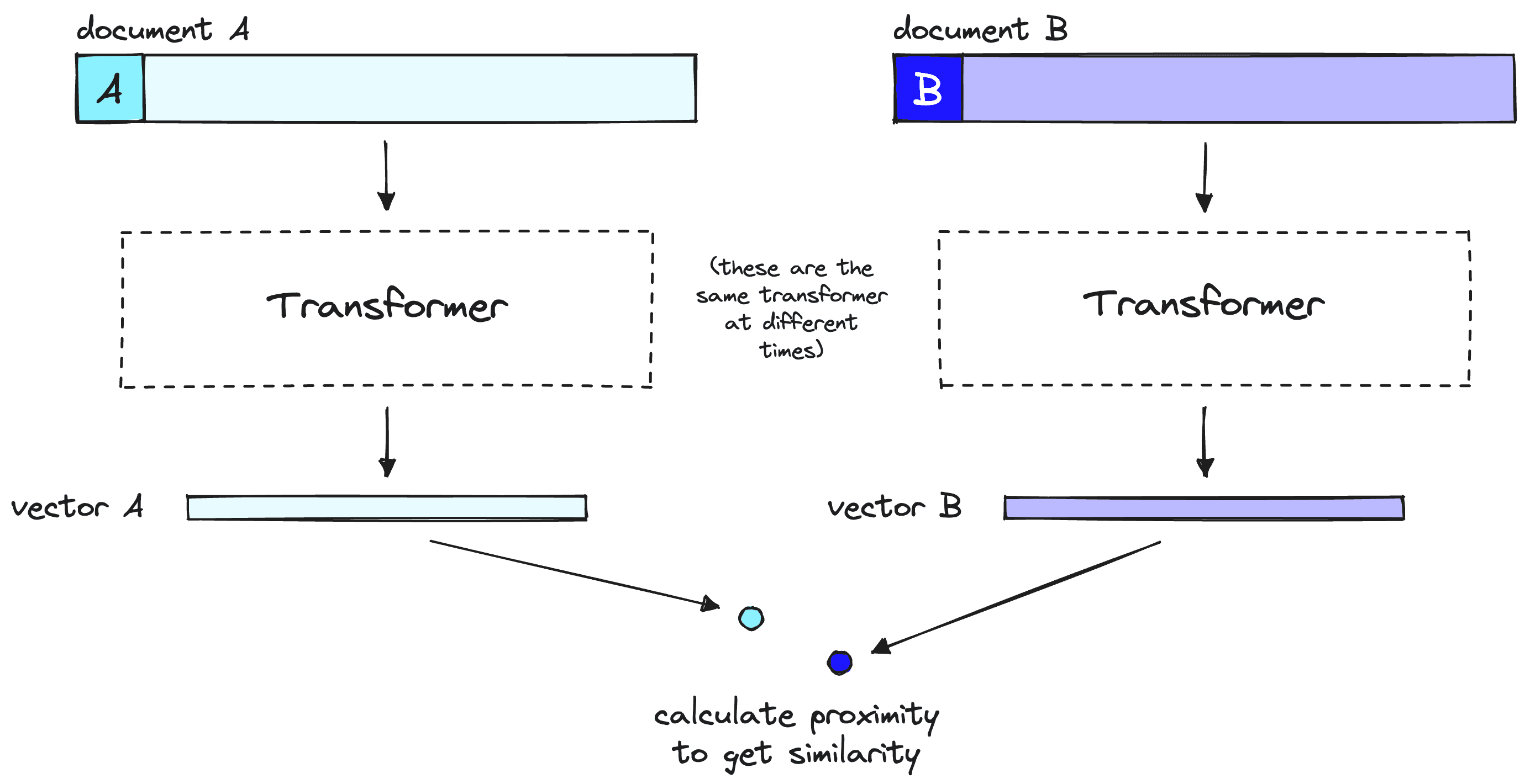
When using bi-encoder models with vector search, we frontload all of the heavy transformer computation to when we are creating the initial vectors — that means that when a user queries our system, we have already created the vectors, so all we need to do is:

1. Run a single transformer computation to create the query vector.
2. Compare the query vector to document vectors with cosine similarity (or another lightweight metric).

With rerankers, we are not pre-computing anything. Instead, we're feeding our query and a single other document into the transformer, running a whole transformer inference step, and outputting a single similarity score.

A reranker considers query and document to produce a single similarity score over a full transformer inference step. Note that document A here is equivalent to our query.

Given 40M records, if we use a small reranking model like BERT on a V100 GPU — we'd be waiting more than 50 hours to return a single query result [3]. We can do the same in <100ms with encoder models and vector search.

Implementing Two-Stage Retrieval with Reranking

Now that we understand the idea and reason behind two-stage retrieval with rerankers, let's see how to implement it (you can follow along with this notebook. To begin we will set up our prerequisite libraries:

!pip install -qU \
  datasets==2.14.5 \
  openai==0.28.1 \
  pinecone-client==2.2.4 \
  cohere==4.27

Data Preparation

Before setting up the retrieval pipeline, we need data to retrieve! We will use the jamescalam/ai-arxiv-chunked dataset from Hugging Face Datasets. This dataset contains more than 400 ArXiv papers on ML, NLP, and LLMs — including the Llama 2, GPTQ, and GPT-4 papers.

The dataset contains 41.5K pre-chunked records. Each record is 1-2 paragraphs long and includes additional metadata about the paper from which it comes. Here is an example:

We'll be feeding this data into Pinecone, so let's reformat the dataset to be more Pinecone-friendly when it does come to the later embed and index process. The format will contain id, text (which we will embed), and metadata. For this example, we won't use metadata, but it can be helpful to include if we want to do metadata filtering in the future.

Embed and Index

To store everything in the vector DB, we need to encode everything with an embedding / bi-encoder model. For simplicity, we will use text-embedding-ada-002 from OpenAI. We do need an OpenAI API key]() to authenticate ourselves via the OpenAI client:

import openai

# platform.openai.com
# get API key from top-right dropdown on OpenAI website
openai.api_key = "YOUR_OPENAI_API_KEY"

embed_model = "text-embedding-ada-002"

Now, we create our vector DB to store our vectors. For this, we need to get a free Pinecone API key — you can find the API key and environment variable in the "API Keys" section of the left navbar.

import pinecone

# initialize connection to pinecone (get API key at app.pinecone.io)
api_key = "YOUR_PINECONE_API_KEY"
# find your environment next to the api key in pinecone console
env = "YOUR_PINECONE_ENV"

pinecone.init(api_key=api_key, environment=env)

After authentication, we create our index. We set dimension equal to the dimensionality of Ada-002 (1536) and use a metric compatible with Ada-002 — that can be either cosine or dotproduct.

import time

index_name = "rerankers"

# check if index already exists (it shouldn't if this is first time)
if index_name not in pinecone.list_indexes():
    # if does not exist, create index
    pinecone.create_index(
        index_name,
        dimension=1536,  # dimensionality of ada 002
        metric='dotproduct'
    )
    # wait for index to be initialized
    while not pinecone.describe_index(index_name).status['ready']:
        time.sleep(1)

# connect to index
index = pinecone.Index(index_name)

We're now ready to begin populating the index using OpenAI's embedding model like so:

from tqdm.auto import tqdm

batch_size = 100  # how many embeddings we create and insert at once

for i in tqdm(range(0, len(data), batch_size)):
    passed = False
    # find end of batch
    i_end = min(len(data), i+batch_size)
    # create batch
    batch = data[i:i_end]
    # create embeddings (exponential backoff to avoid RateLimitError)
    for j in range(5):  # max 5 retries
        try:
            res = openai.Embedding.create(input=batch["text"], engine=embed_model)
            passed = True
        except openai.error.RateLimitError:
            time.sleep(2**j)  # wait 2^j seconds before retrying
            print("Retrying...")
    if not passed:
        raise RuntimeError("Failed to create embeddings.")
    # get embeddings
    embeds = [record['embedding'] for record in res['data']]
    to_upsert = list(zip(batch["id"], embeds, batch["metadata"]))
    # upsert to Pinecone
    index.upsert(vectors=to_upsert)

Our index is now populated and ready for us to query!

Retrieval Without Reranking

Before reranking, let's see how our results look without it. We will define a function called get_docs to return documents using the first stage of retrieval only:

def get_docs(query: str, top_k: int):
    # encode query
    xq = embed([query])[0]
    # search pinecone index
    res = index.query(xq, top_k=top_k, include_metadata=True)
    # get doc text
    docs = {x["metadata"]['text']: i for i, x in enumerate(res["matches"])}
    return docs

Let's ask about Reinforcement Learning with Human Feedback — a popular fine-tuning method behind the sudden performance gains demonstrated by ChatGPT when it was released.

We get reasonable performance here — notably relevant chunks of text:

The remaining documents and text cover RLHF but don't answer our specific question of "why we would want to do rlhf?".

Reranking Responses

We will use Cohere's rerank endpoint for reranking. You will need a Cohere API key to use it. With our API key, we authenticate like so:

import cohere

# init client
co = cohere.Client("YOUR_COHERE_API_KEY")

Now, we can rerank our results with co.rerank. Let's try increasing the number of results returned by the first-stage retrieval step to a top_k=25 and reranking them all (setting top_n=25) to see what the reordering we get looks like.

We still have record 0 at the top — that is great because it contained plenty of relevant information to our query. However, the less relevant documents 1 and 2 have been replaced by documents 23 and 14, respectively.

Let's create a function that will allow us to compare original vs. reranked results more quickly.

def compare(query: str, top_k: int, top_n: int):
    # first get vec search results
    docs = get_docs(query, top_k=top_k)
    i2doc = {docs[doc]: doc for doc in docs.keys()}
    # rerank
    rerank_docs = co.rerank(
        query=query, documents=docs.keys(), top_n=top_n, model="rerank-english-v2.0"
    )
    original_docs = []
    reranked_docs = []
    # compare order change
    for i, doc in enumerate(rerank_docs):
        rerank_i = docs[doc.document["text"]]
        print(str(i)+"\t->\t"+str(rerank_i))
        if i != rerank_i:
            reranked_docs.append(f"[{rerank_i}]\n"+doc.document["text"])
            original_docs.append(f"[{i}]\n"+i2doc[i])
    for orig, rerank in zip(original_docs, reranked_docs):
        print("ORIGINAL:\n"+orig+"\n\nRERANKED:\n"+rerank+"\n\n---\n")

We start with our RLHF query. This time, we do a more standard retrieval-rerank process of retrieving 25 documents (top_k=25) and reranking to the top three documents (top_n=3).

Looking at these, we have dropped the one relevant chunk of text from document 1 and no relevant chunks of text from document 2 — the following relevant pieces of information now replace these:

We have far more relevant information after reranking. Naturally, this can result in significantly better performance for RAG. It means we maximize relevant information while minimizing noise input into our LLM.

Reranking is one of the simplest methods for dramatically improving recall performance in Retrieval Augmented Generation (RAG) or any other retrieval-based pipeline.

We've explored why rerankers can provide so much better performance than their embedding model counterparts — and how a two-stage retrieval system allows us to get the best of both, enabling search at scale while maintaining quality performance.

References

[1] Introducing 100K Context Windows (2023), Anthropic

[2] N. Liu, K. Lin, J. Hewitt, A. Paranjape, M. Bevilacqua, F. Petroni, P. Liang, Lost in the Middle: How Language Models Use Long Contexts (2023),

[3] N. Reimers, I. Gurevych, Sentence-BERT: Sentence Embeddings using Siamese BERT-Networks (2019), UKP-TUDA