Semantic Search: Measuring Meaning From Jaccard to Bert

Similarity search is one of the fastest-growing domains in AI and machine learning. At its core, it is the process of matching relevant pieces of information together.

There’s a strong chance that you found this article through a search engine — most likely Google. Maybe you searched something like “what is semantic similarity search?” or “traditional vs vector similarity search”.

Google processed your query and used many of the same similarity search essentials that we will learn about in this article, to bring you to — this article.

Note: Want to replace your keyword search with semantic search powered by NLP? Pinecone makes it easy, scalable, and free — start now.

If similarity search is at the heart of the success of a $1.65T company — the world’s fifth most valuable company in the world[1], there’s a good chance it’s worth learning more about.

Similarity search is a complex topic and there are countless techniques for building effective search engines.

In this article, we’ll cover a few of the most interesting — and powerful — of these techniques — focusing specifically on semantic search. We’ll learn how they work, what they’re good at, and how we can implement them ourselves.

Watch the videos or continue reading:

Traditional Search

We start our journey down the road of search in the traditional camp, here we find a few key players like:

• Jaccard Similarity
• w-shingling
• Pearson Similarity
• Levenshtein distance
• Normalized Google Distance

All are great metrics to use with similarity search — of which we’ll cover three of the most popular, Jaccard similarity, w-shingling, and Levenshtein distance.

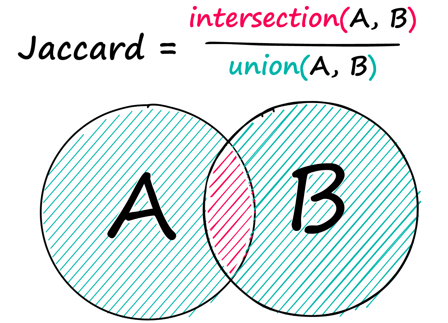
Jaccard Similarity

Jaccard similarity is a simple, but sometimes powerful similarity metric. Given two sequences, A and B — we find the number of shared elements between both and divide this by the total number of elements from both sequences.

Jaccard similarity measures the intersection between two sequences over the union between the two sequences.

Given two sequences of integers, we would write:

a = [0, 1, 2, 3, 3, 3, 4]
b = [7, 6, 5, 4, 4, 3]

# convert to sets
a = set(a)
b = set(b)

a

{0, 1, 2, 3, 4}

# find the number of shared values between sets
shared = a.intersection(b)
shared

{3, 4}

# find the total number of values in both sets
total = a.union(b)
total

{0, 1, 2, 3, 4, 5, 6, 7}

# and calculate Jaccard similarity
len(shared) / len(total)

0.25

Here we identified two shared unique integers, 3 and 4 — between two sequences with a total of ten integers in both, of which eight are unique values — 2/8 gives us our Jaccard similarity score of 0.25.

We could perform the same operation for text data too, all we do is replace integers with tokens.

Jaccard similarity calculated between two sentences a and b.

a = "his thought process was on so many levels that he gave himself a phobia of heights".split()
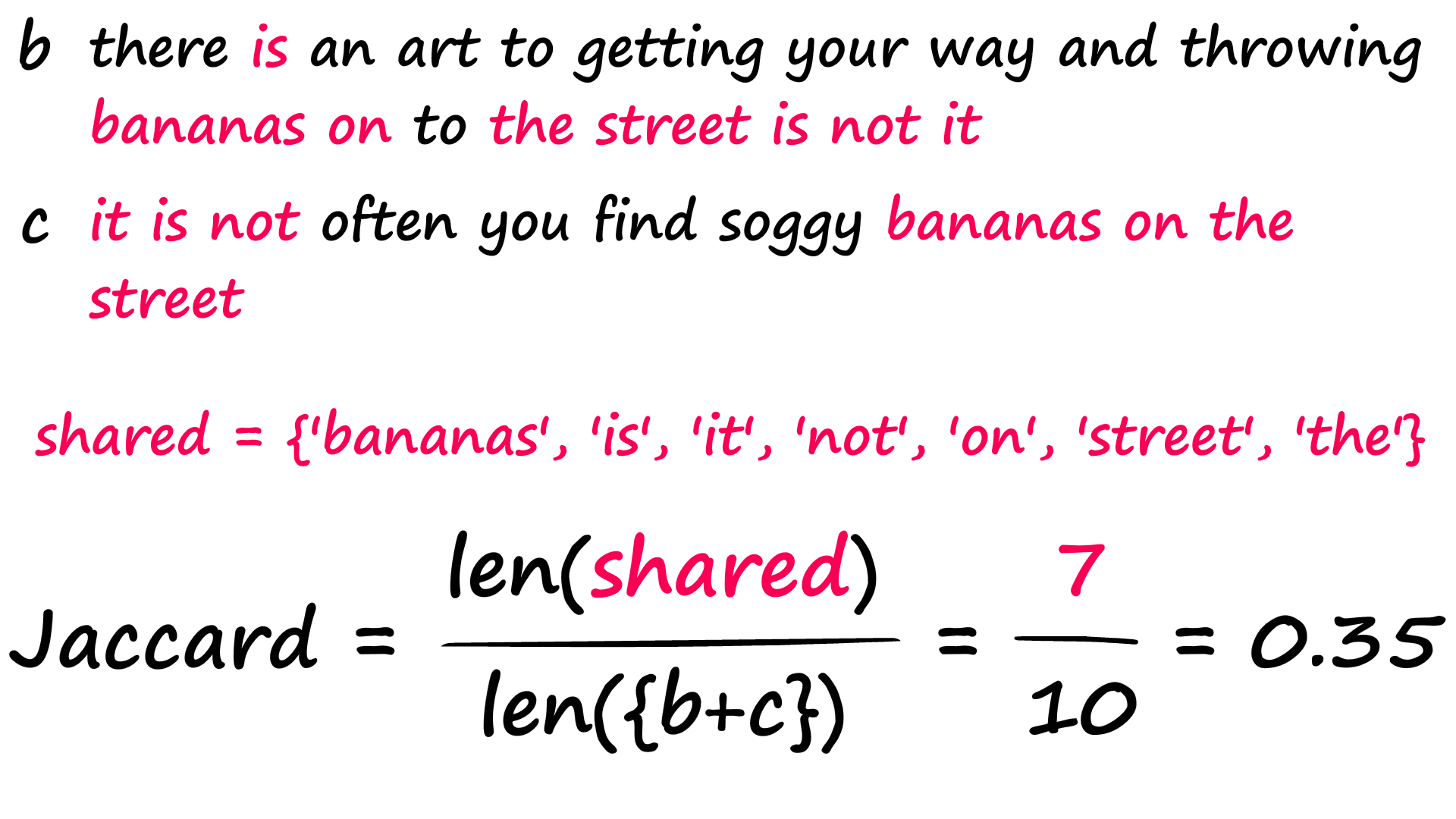
b = "there is an art to getting your way and throwing bananas on to the street is not it".split()
c = "it is not often you find soggy bananas on the street".split()

print(c)

['it', 'is', 'not', 'often', 'you', 'find', 'soggy', 'bananas', 'on', 'the', 'street']

Convert our lists into sets (removing any duplication of words).

a = set(a)
b = set(b)
c = set(c)

print(c)

{'you', 'the', 'often', 'street', 'not', 'it', 'find', 'is', 'on', 'soggy', 'bananas'}

And now calculate our Jaccard similarity - which we can write as a function.

def jac(x: set, y: set):
    shared = x.intersection(y)  # selects shared tokens only
    return len(shared) / len(x.union(y))  # union adds both sets together

jac(a, b)

0.03225806451612903

jac(b, c)

0.35

We find that sentences b and c score much better, as we would expect. Now, it isn’t perfect — two sentences that share nothing but words like ‘the’, ‘a’, ‘is’, etc — could return high Jaccard scores despite being semantically dissimilar.

These shortcomings can be solved partially using preprocessing techniques like stopword removal, stemming/lemmatization, and so on. However, as we’ll see soon — some methods avoid these problems altogether.

w-Shingling

Another similar technique is w-shingling. w-shingling uses the exact same logic of intersection / union — but with ‘shingles’. A 2-shingle of sentence a would look something like:

a = {'his thought', 'thought process', 'process is', ...}

We would then use the same calculation of intersection / union between our shingled sentences like so:

a = "his thought process was on so many levels that he gave himself a phobia of heights".split()
b = "there is an art to getting your way and throwing bananas on to the street is not it".split()
c = "it is not often you find soggy bananas on the street".split()

a_shingle = set([' '.join([a[i], a[i+1]]) for i in range(len(a)) if i != len(a)-1])
b_shingle = set([' '.join([b[i], b[i+1]]) for i in range(len(b)) if i != len(b)-1])
c_shingle = set([' '.join([c[i], c[i+1]]) for i in range(len(c)) if i != len(c)-1])
print(a_shingle)

{'he gave', 'gave himself', 'phobia of', 'on so', 'many levels', 'thought process', 'himself a', 'process was', 'a phobia', 'was on', 'his thought', 'that he', 'of heights', 'levels that', 'so many'}

jac(a_shingle, b_shingle)  # we use the exact same Jaccard similarity calculation

0.0

jac(b_shingle, c_shingle)

0.125

b_shingle.intersection(c_shingle)  # these are the matching shingles

{'bananas on', 'is not', 'the street'}

Using a 2-shingle, we find three matching shingles between sentences b and c, resulting in a similarity of 0.125.

Levenshtein Distance

Another popular metric for comparing two strings is the Levenshtein distance. It is calculated as the number of operations required to change one string into another — and it’s calculated with:

Levenshtein distance formula.

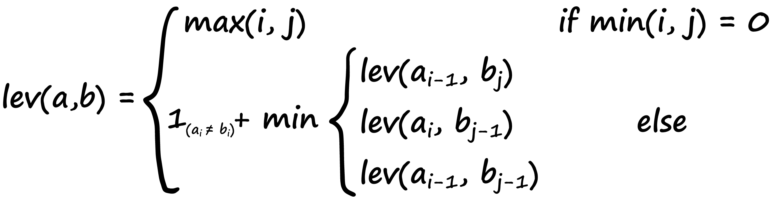
Now, this is a pretty complicated-looking formula — if you understand it, great! If not, don’t worry — we’ll break it down.

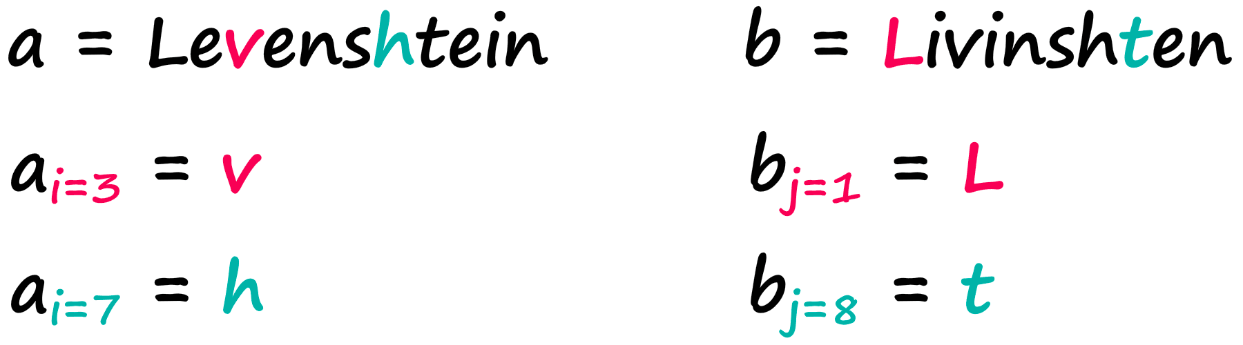
The variables a and b represent our two strings, i and j represent the character position in a and b respectively. So given the strings:

‘Levenshtein’ and a mispelling ‘Livinshten’.

We would find:

We index the word itself from 1 to the length of the word, the zeroth index does exist as a none character (more on that next).

Easy! Now, a great way to grasp the logic behind this formula is through visualizing the Wagner-Fischer algorithm — which uses a simple matrix to calculate our Levenshtein distance.

We take our two words a and b and place them on either axis of our matrix — we include our none character as an empty space.

Our empty Wagner-Fischer matrix — we’ll be using this to calculate the Levenshtein distance between ‘Levenshtein’ and ‘Livinshten’.

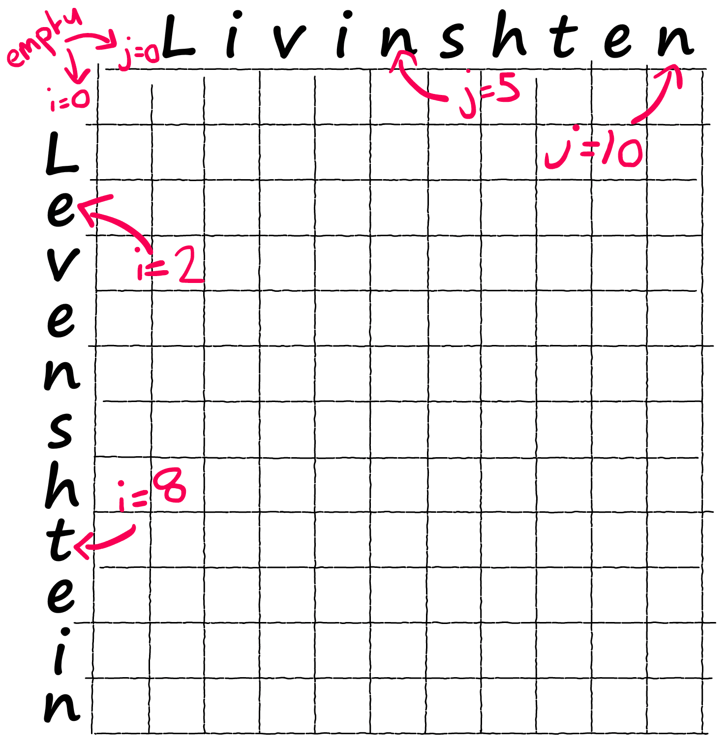
a = ' Levenshtein'
b = ' Livinshten'  # we include empty space at start of each word

import numpy as np
# initialize empty zero array
lev = np.zeros((len(a), len(b)))
lev

array([[0., 0., 0., 0., 0., 0., 0., 0., 0., 0., 0.],
       [0., 0., 0., 0., 0., 0., 0., 0., 0., 0., 0.],
       [0., 0., 0., 0., 0., 0., 0., 0., 0., 0., 0.],
       [0., 0., 0., 0., 0., 0., 0., 0., 0., 0., 0.],
       [0., 0., 0., 0., 0., 0., 0., 0., 0., 0., 0.],
       [0., 0., 0., 0., 0., 0., 0., 0., 0., 0., 0.],
       [0., 0., 0., 0., 0., 0., 0., 0., 0., 0., 0.],
       [0., 0., 0., 0., 0., 0., 0., 0., 0., 0., 0.],
       [0., 0., 0., 0., 0., 0., 0., 0., 0., 0., 0.],
       [0., 0., 0., 0., 0., 0., 0., 0., 0., 0., 0.],
       [0., 0., 0., 0., 0., 0., 0., 0., 0., 0., 0.],
       [0., 0., 0., 0., 0., 0., 0., 0., 0., 0., 0.]])

Then we iterate through every position in our matrix and apply that complicated formula we saw before.

The first step in our formulae is if min(i, j) = 0 — all we’re saying here is, out of our two positions i and j, are either 0? If so, we move across to max(i, j) which tells us to assign the current position in our matrix the higher of the two positions i and j:

We start on the right, along the edges where i and/or j is 0, the matrix position will be populated with max(i, j).

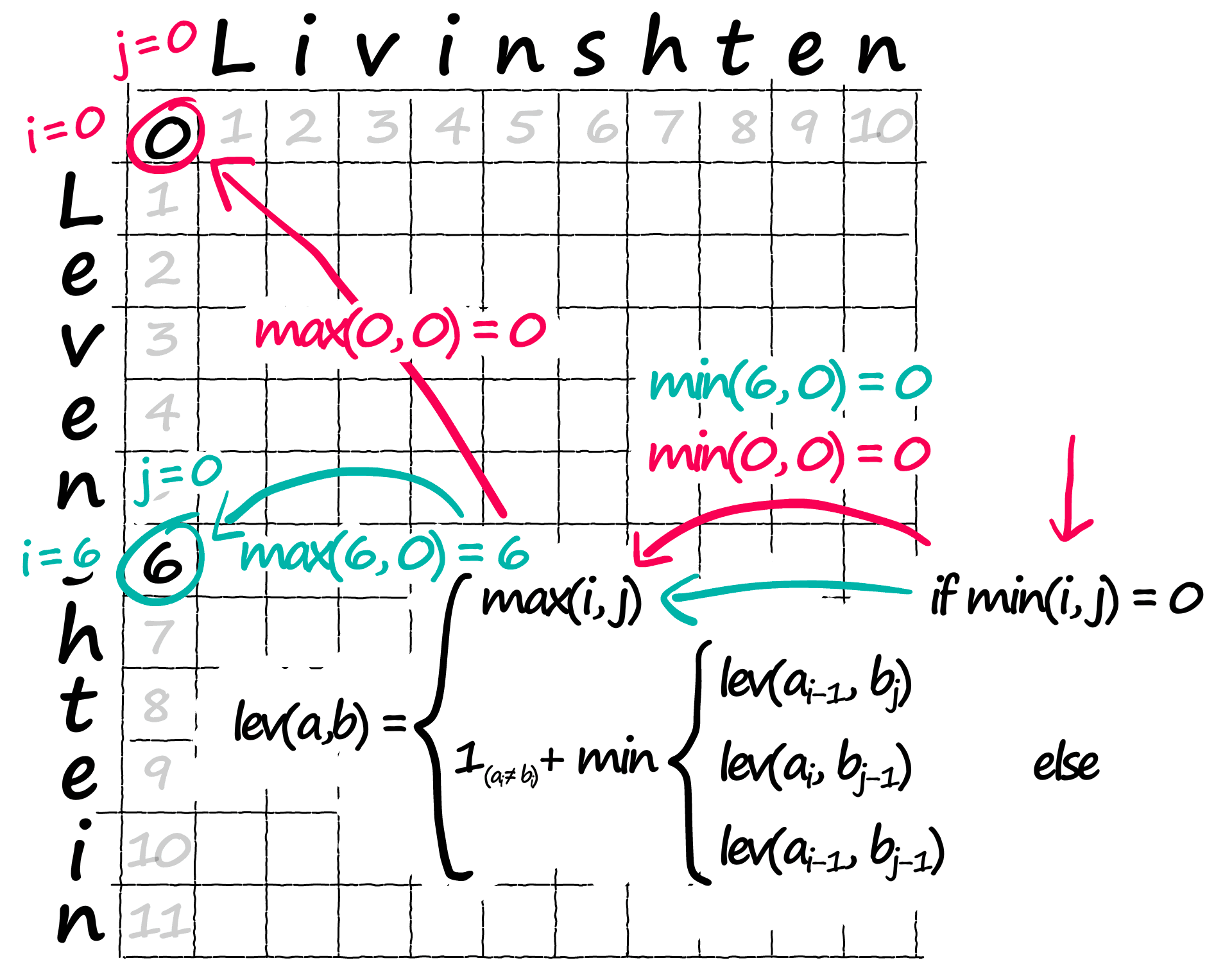
for i in range(len(a)):
    for j in range(len(b)):
        # if i or j are 0
        if min([i, j]) == 0:
            # we assign matrix value at position i, j = max(i, j)
            lev[i, j] = max([i, j])
lev

array([[ 0.,  1.,  2.,  3.,  4.,  5.,  6.,  7.,  8.,  9., 10.],
       [ 1.,  0.,  0.,  0.,  0.,  0.,  0.,  0.,  0.,  0.,  0.],
       [ 2.,  0.,  0.,  0.,  0.,  0.,  0.,  0.,  0.,  0.,  0.],
       [ 3.,  0.,  0.,  0.,  0.,  0.,  0.,  0.,  0.,  0.,  0.],
       [ 4.,  0.,  0.,  0.,  0.,  0.,  0.,  0.,  0.,  0.,  0.],
       [ 5.,  0.,  0.,  0.,  0.,  0.,  0.,  0.,  0.,  0.,  0.],
       [ 6.,  0.,  0.,  0.,  0.,  0.,  0.,  0.,  0.,  0.,  0.],
       [ 7.,  0.,  0.,  0.,  0.,  0.,  0.,  0.,  0.,  0.,  0.],
       [ 8.,  0.,  0.,  0.,  0.,  0.,  0.,  0.,  0.,  0.,  0.],
       [ 9.,  0.,  0.,  0.,  0.,  0.,  0.,  0.,  0.,  0.,  0.],
       [10.,  0.,  0.,  0.,  0.,  0.,  0.,  0.,  0.,  0.,  0.],
       [11.,  0.,  0.,  0.,  0.,  0.,  0.,  0.,  0.,  0.,  0.]])

Now, we’ve dealt with the outer edges of our matrix — but we still need to calculate the inner values — which is where our optimal path will be found.

Back to if min(i, j) = 0 — what if neither are 0? Then we move onto that complex part of the equation inside the min { section. We need to calculate a value for each row, then we take the minimum value.

Now, we already know these values — they’re in our matrix:

For each new position in our matrix, we take the minimum value from the three neighboring positions (circled — top-left).

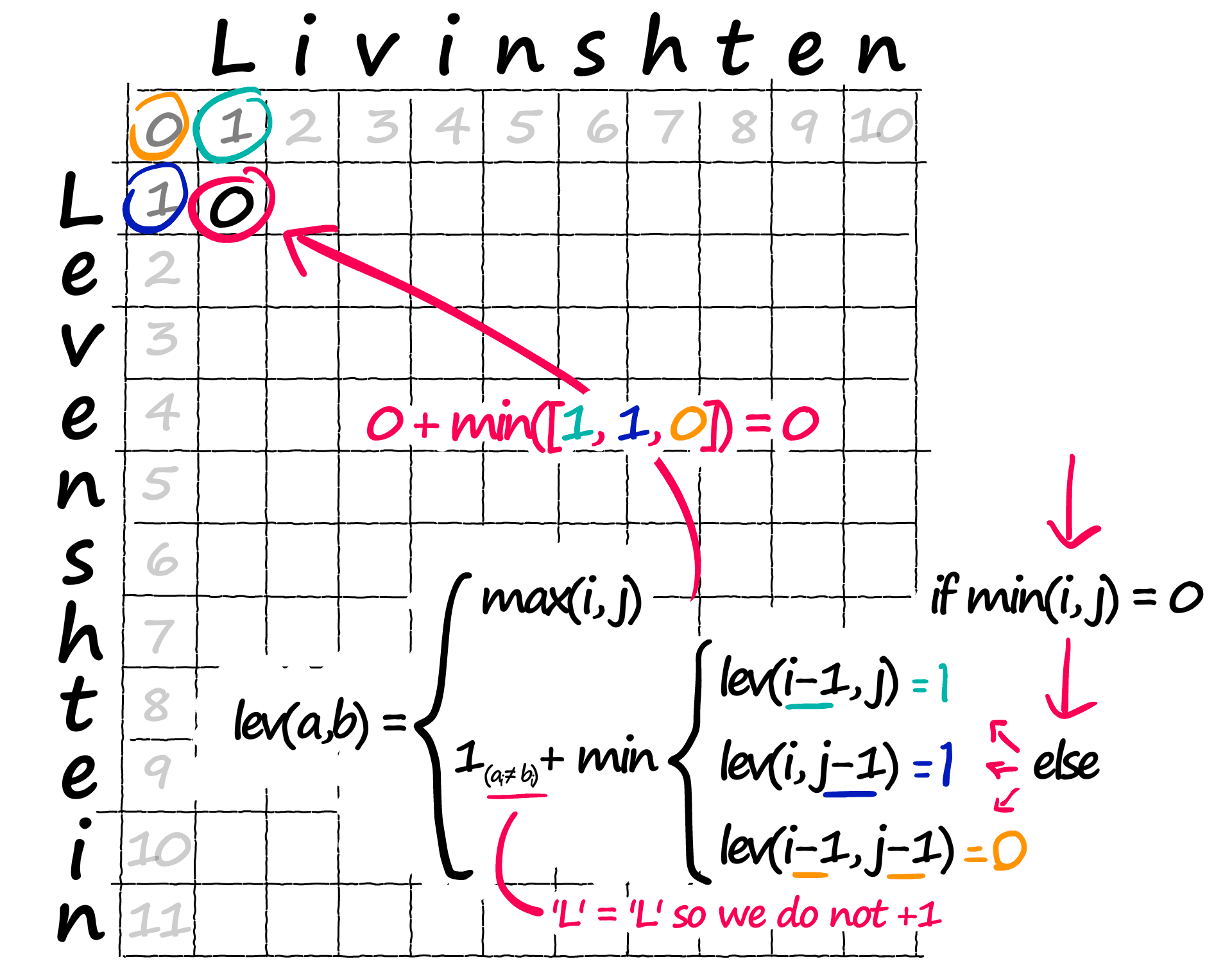
lev(i-1, j) and the other operations are all indexing operations — where we extract the value in that position. We then take the minimum value of the three.

There is just one remaining operation. The +1 on the left should only be applied if a[i] != b[i] — this is the penalty for mismatched characters.

If a[i] != b[j] we add 1 to our minimum value — this is the penalty for mismatched characters.

Placing all of this together into an iterative loop through the full matrix looks like this:

for i in range(len(a)):
    for j in range(len(b)):
        # we did this before (for when i or j are 0)
        if min([i, j]) == 0:
            lev[i, j] = max([i, j])
        else:
            # calculate our three possible operations
            x = lev[i-1, j]  # deletion
            y = lev[i, j-1]  # insertion
            z = lev[i-1, j-1]  # substitution
            # take the minimum (eg best path/operation)
            lev[i, j] = min([x, y, z])
            # and if our two current characters don't match, add 1
            if a[i] != b[j]:
                # if we have a match, don't add 1
                lev[i, j] += 1
lev

array([[ 0.,  1.,  2.,  3.,  4.,  5.,  6.,  7.,  8.,  9., 10.],
       [ 1.,  0.,  1.,  2.,  3.,  4.,  5.,  6.,  7.,  8.,  9.],
       [ 2.,  1.,  1.,  2.,  3.,  4.,  5.,  6.,  7.,  7.,  8.],
       [ 3.,  2.,  2.,  1.,  2.,  3.,  4.,  5.,  6.,  7.,  8.],
       [ 4.,  3.,  3.,  2.,  2.,  3.,  4.,  5.,  6.,  6.,  7.],
       [ 5.,  4.,  4.,  3.,  3.,  2.,  3.,  4.,  5.,  6.,  6.],
       [ 6.,  5.,  5.,  4.,  4.,  3.,  2.,  3.,  4.,  5.,  6.],
       [ 7.,  6.,  6.,  5.,  5.,  4.,  3.,  2.,  3.,  4.,  5.],
       [ 8.,  7.,  7.,  6.,  6.,  5.,  4.,  3.,  2.,  3.,  4.],
       [ 9.,  8.,  8.,  7.,  7.,  6.,  5.,  4.,  3.,  2.,  3.],
       [10.,  9.,  8.,  8.,  7.,  7.,  6.,  5.,  4.,  3.,  3.],
       [11., 10.,  9.,  9.,  8.,  7.,  7.,  6.,  5.,  4.,  3.]])

We’ve now calculated each value in the matrix — these represent the number of operations required to convert from string a up to position i to string b up to position j.

We’re looking for the number of operations to convert a to b — so we take the bottom-right value of our array at lev[-1, -1].

The optimal path through our matrix — in position [-1, -1] at the bottom-right we have the Levenshtein distance between our two strings.

lev[-1, -1]

3.0

Vector Similarity Search

For vector-based search, we typically find one of several vector building methods:

• TF-IDF
• BM25
• word2vec/doc2vec
• BERT
• USE

In tandem with some implementation of approximate nearest neighbors (ANN), these vector-based methods are the MVPs in the world of similarity search.

We’ll cover TF-IDF, BM25, and BERT-based approaches — as these are easily the most common and cover both sparse and dense vector representations.

1. TF-IDF

The respected grandfather of vector similarity search, born back in the 1970s. It consists of two parts, Term Frequency (TF) and Inverse Document Frequency (IDF).

The TF component counts the number of times a term appears within a document and divides this by the total number of terms in that same document.

The term frequency (TF) component of TF-IDF counts the frequency of our query (‘bananas’) and divides by the frequency of all tokens.

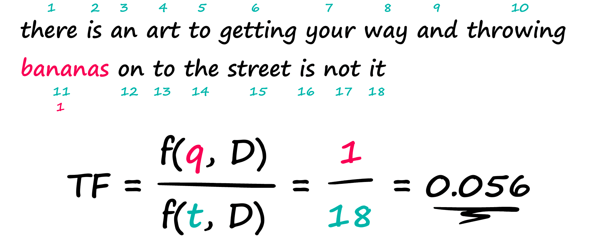
That is the first half of our calculation, we have the frequency of our query within the current Document f(q,D) — over the frequency of all terms within the current Document f(t,D).

The Term Frequency is a good measure, but doesn’t allow us to differentiate between common and uncommon words. If we were to search for the word ‘the’ — using TF alone we’d assign this sentence the same relevance as had we searched ‘bananas’.

That’s fine until we begin comparing documents, or searching with longer queries. We don’t want words like ‘the’,_ ‘is’_, or _‘it’_ to be ranked as highly as _‘bananas’_ or _‘street’_.

Ideally, we want matches between rarer words to score higher. To do this, we can multiply TF by the second term — IDF. The Inverse Document Frequency measures how common a word is across all of our documents.

The inverse document frequency (IDF) component of TF-IDF counts the number of documents that contain our query.

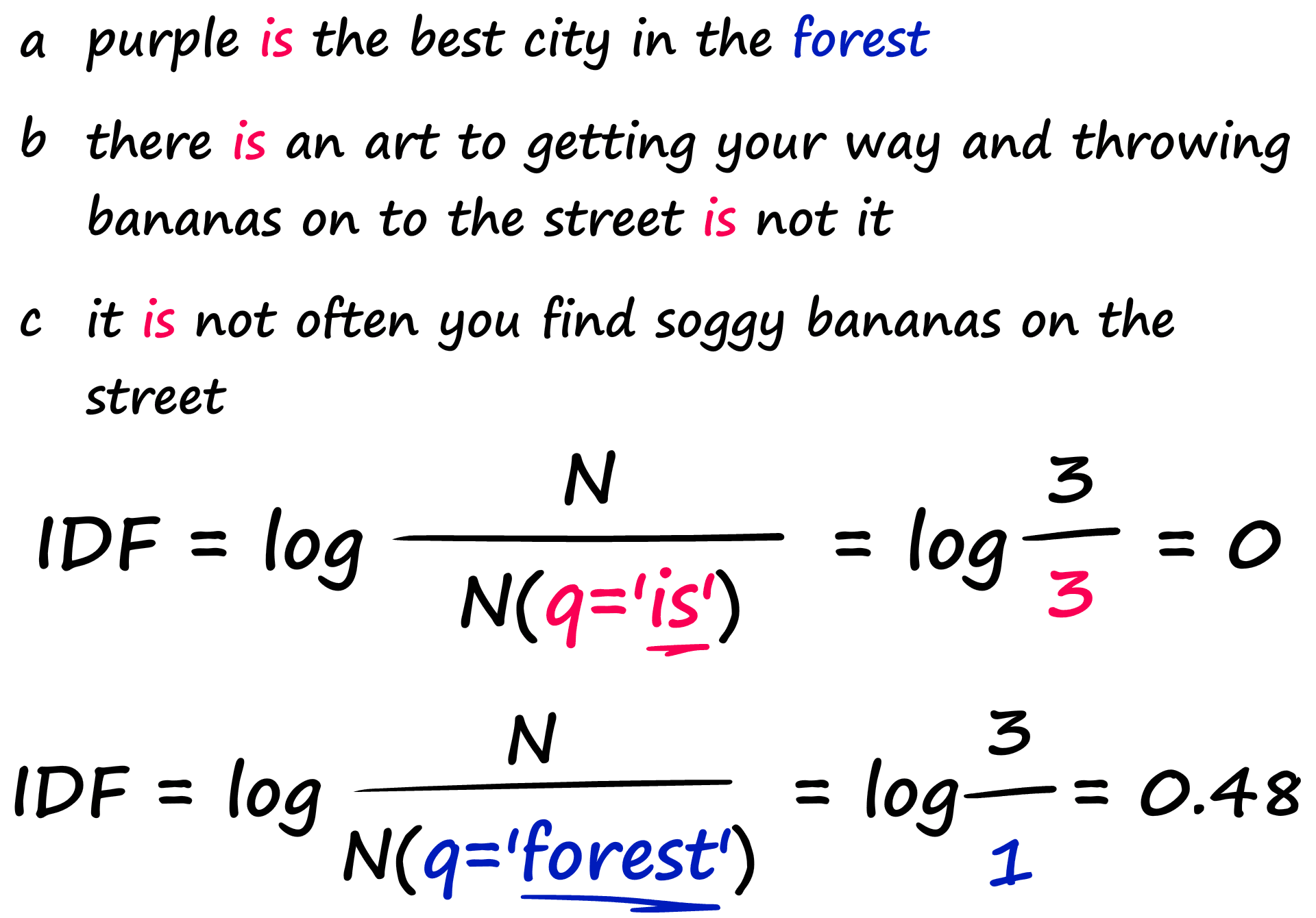
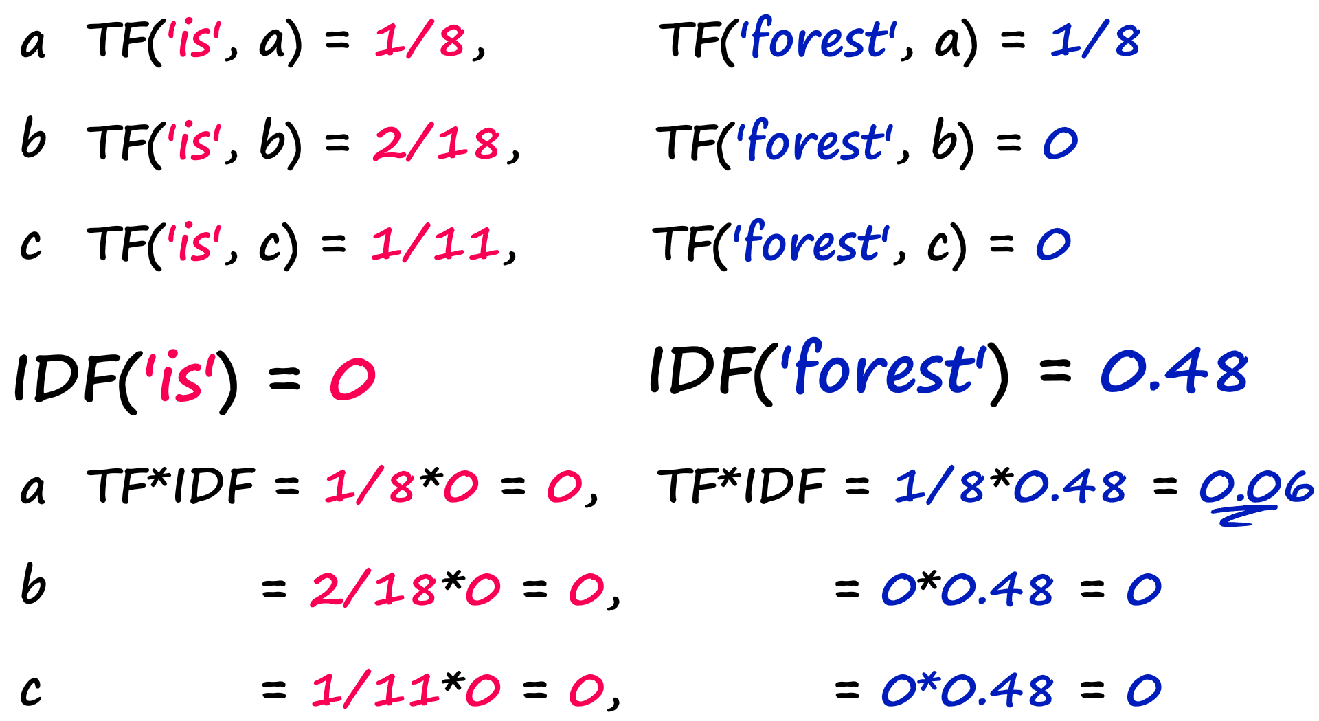
In this example, we have three sentences. When we calculate the IDF for our common word ‘is’, we return a much lower number than that for the rarer word ‘forest’.

If we were to then search for both words ‘is’ and ‘forest’ we would merge TF and IDF like so:

We calculate the TF(‘is’, D) and TF(‘forest’, D) scores for docs a, b, and c. The IDF value is across all docs — so we calculate just IDF(‘is’) and IDF(‘forest’) once. Then, we get TF-IDF values for both words in each doc by multiplying the TF and IDF components. Sentence a scores highest for ‘forest’, and ‘is’ always scores 0 as the IDF(‘is’) score is 0.

a = "purple is the best city in the forest".split()
b = "there is an art to getting your way and throwing bananas on to the street is not it".split()
c = "it is not often you find soggy bananas on the street".split()

import numpy as np

def tfidf(word):
    tf = []
    count_n = 0
    for sentence in [a, b, c]:
        # calculate TF
        t_count = len([x for x in sentence if word in sentence])
        tf.append(t_count/len(sentence))
        # count number of docs for IDF
        count_n += 1 if word in sentence else 0
    idf = np.log10(len([a, b, c]) / count_n)
    return [round(_tf*idf, 2) for _tf in tf]

tfidf_a, tfidf_b, tfidf_c = tfidf('forest')
print(f"TF-IDF a: {tfidf_a}\nTF-IDF b: {tfidf_b}\nTF-IDF c: {tfidf_c}")

TF-IDF a: 0.48
TF-IDF b: 0.0
TF-IDF c: 0.0

That’s great, but where does vector similarity search come into this? Well, we take our vocabulary (a big list of all words in our dataset) — and calculate the TF-IDF for each and every word.

We calculate the TF-IDF value for every word in our vocabulary to create a TF-IDF vector. This process is repeated for each document.

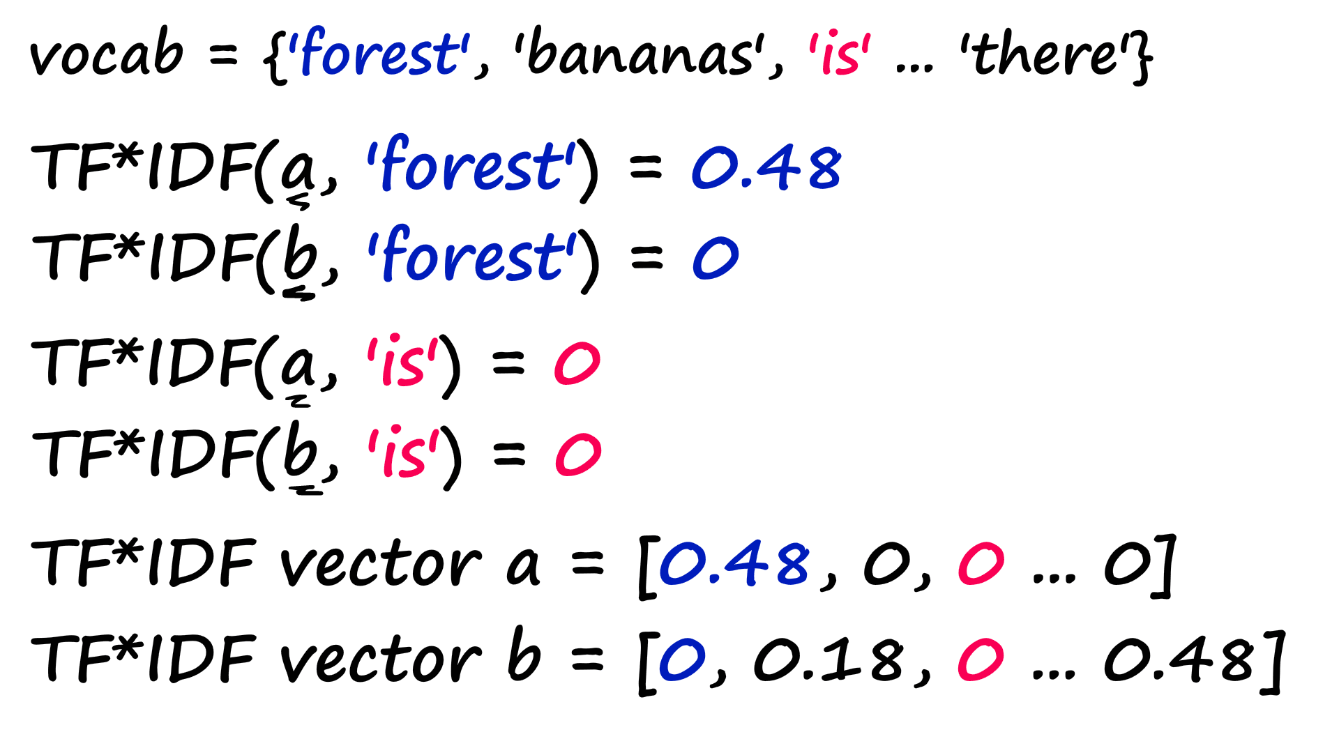
We can put all of this together to create our TF-IDF vectors like so:

vocab = set(a+b+c)

print(vocab)

{'an', 'and', 'street', 'is', 'on', 'best', 'way', 'there', 'forest', 'often', 'in', 'purple', 'throwing', 'you', 'art', 'your', 'city', 'find', 'the', 'not', 'soggy', 'it', 'getting', 'to', 'bananas'}

# initialize vectors
vec_a = []
vec_b = []
vec_c = []

for word in vocab:
    tfidf_a, tfidf_b, tfidf_c = tfidf(word)
    vec_a.append(tfidf_a)
    vec_b.append(tfidf_b)
    vec_c.append(tfidf_c)

print(vec_a)

[0.0, 0.0, 0.0, 0.0, 0.0, 0.48, 0.0, 0.0, 0.48, 0.0, 0.48, 0.48, 0.0, 0.0, 0.0, 0.0, 0.48, 0.0, 0.0, 0.0, 0.0, 0.0, 0.0, 0.0, 0.0]

print(vec_b)

[0.48, 0.48, 0.18, 0.0, 0.18, 0.0, 0.48, 0.48, 0.0, 0.0, 0.0, 0.0, 0.48, 0.0, 0.48, 0.48, 0.0, 0.0, 0.0, 0.18, 0.0, 0.18, 0.48, 0.48, 0.18]

From there we have our TF-IDF vector. It’s worth noting that vocab sizes can easily be in the 20K+ range, so the vectors produced using this method are incredibly sparse — which means we cannot encode any semantic meaning.

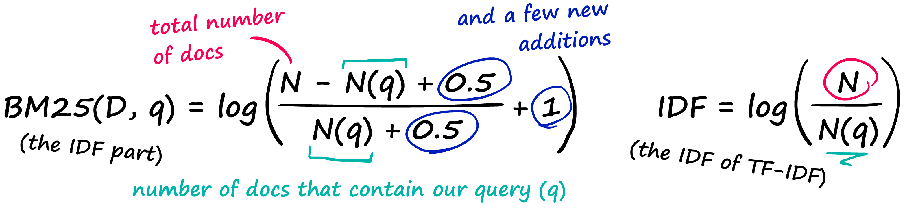
2. BM25

The successor to TF-IDF, Okapi BM25 is the result of optimizing TF-IDF primarily to normalize results based on document length.

TF-IDF is great but can return questionable results when we begin comparing several mentions

If we took two 500 word articles and found that article A mentions ‘Churchill’ six times, and article B mentions ‘Churchill’ twelve times — should we view article A as half as relevant? Likely not.

BM25 solves this by modifying TF-IDF:

The BM25 formula.

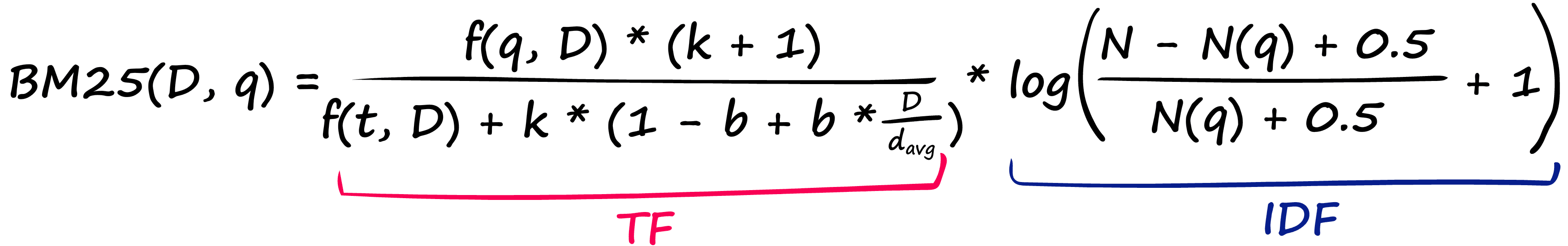
That’s a pretty nasty-looking equation — but it’s nothing more than our TF-IDF formula with a few new parameters! Let’s compare the two TF components:

The TF part of BM25 (left) compared to the TF of TF-IDF (right).

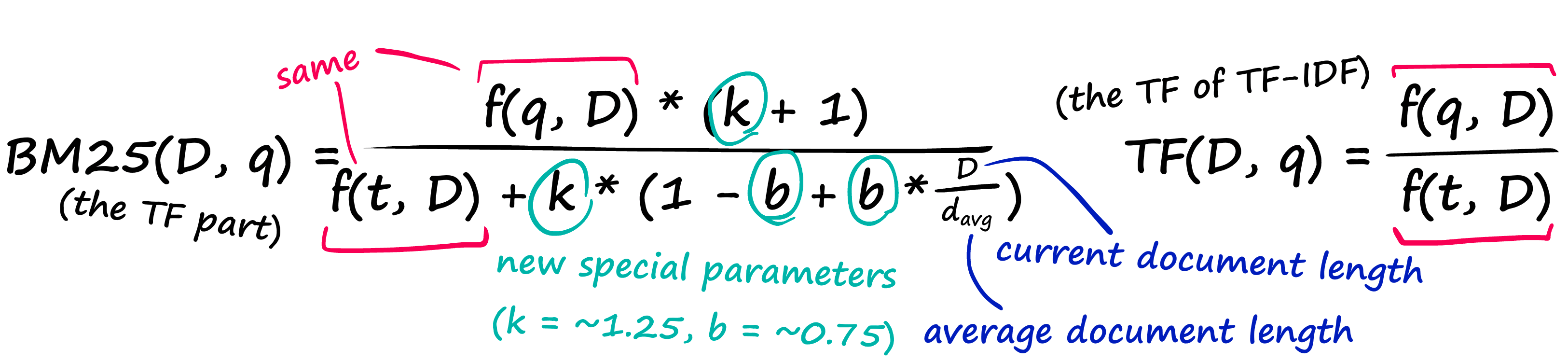
And then we have the IDF part, which doesn’t even introduce any new parameters — it just rearranges our old IDF from TF-IDF.

The IDF part of BM25 (left) compared to the IDF of TF-IDF (right).

Now, what is the result of this modification? If we take a sequence containing 12 tokens, and gradually feed it more and more ‘matching’ tokens — we produce the following scores:

Comparison of TF-IDF (top) and BM25 (bottom) algorithms using a sentence of 12 tokens, and an incremental number of relevant tokens (x-axis).

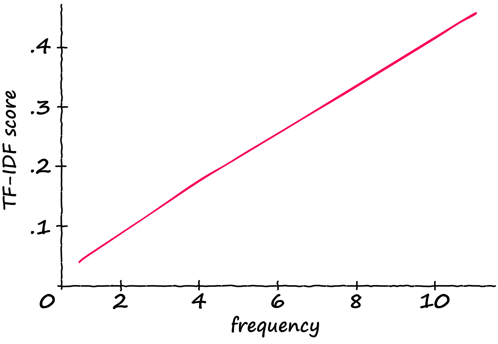
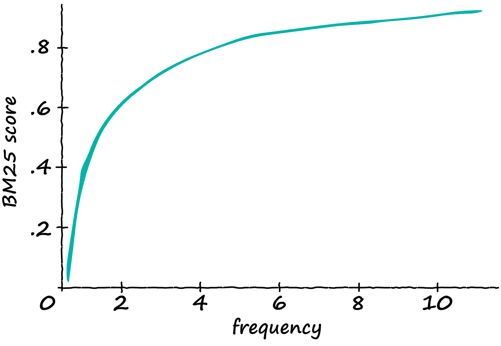
The TF-IDF score increases linearly with the number of relevant tokens. So, if the frequency doubles — so does the TF-IDF score.

Sounds cool! But how do we implement it in Python? Again, we’ll keep it nice and simple like the TF-IDF implementation.

a = "purple is the best city in the forest".split()
b = "there is an art to getting your way and throwing bananas on to the street is not it".split()
c = "it is not often you find soggy bananas on the street".split()
d = "green should have smelled more tranquil but somehow it just tasted rotten".split()
e = "joyce enjoyed eating pancakes with ketchup".split()
f = "as the asteroid hurtled toward earth becky was upset her dentist appointment had been canceled".split()

docs = [a, b, c, d, e, f]

import numpy as np

avgdl = sum(len(sentence) for sentence in [a,b,c,d,e,f]) / len(docs)
N = len(docs)

def bm25(word, sentence, k=1.2, b=0.75):
    freq = sentence.count(word)  # or f(q,D) - freq of query in Doc
    tf = (freq * (k + 1)) / (freq + k * (1 - b + b * (len(sentence) / avgdl)))
    N_q = sum([doc.count(word) for doc in docs])  # number of docs that contain the word
    idf = np.log(((N - N_q + 0.5) / (N_q + 0.5)) + 1)
    return round(tf*idf, 4)

bm25('purple', a)

1.7677

bm25('purple', b)

0.0

bm25('bananas', b)

0.8425

bm25('bananas', c)

1.0543

We’ve used the default parameters for k and b — and our outputs look promising. The query 'purple' only matches sentence a, and 'bananas' scores reasonable for both b and c — but slightly higher in c thanks to the smaller word count.

To build vectors from this, we do the exact same thing we did for TF-IDF.

vocab = set(a+b+c+d+e+f)
print(vocab)

{'it', 'is', 'and', 'just', 'should', 'becky', 'have', 'you', 'there', 'had', 'getting', 'as', 'not', 'green', 'was', 'an', 'ketchup', 'earth', 'more', 'rotten', 'smelled', 'toward', 'enjoyed', 'in', 'bananas', 'on', 'often', 'street', 'forest', 'with', 'throwing', 'city', 'eating', 'canceled', 'soggy', 'somehow', 'dentist', 'but', 'tasted', 'pancakes', 'hurtled', 'to', 'asteroid', 'upset', 'art', 'the', 'her', 'been', 'best', 'way', 'joyce', 'appointment', 'your', 'purple', 'tranquil', 'find'}

vec = []
# we will create the BM25 vector for sentence 'a'
for word in vocab:
    vec.append(bm25(word, a))
print(vec)

[0.0, 0.507, 0.0, 0.0, 0.0, 0.0, 0.0, 0.0, 0.0, 0.0, 0.0, 0.0, 0.0, 0.0, 0.0, 0.0, 0.0, 0.0, 0.0, 0.0, 0.0, 0.0, 0.0, 1.7677, 0.0, 0.0, 0.0, 0.0, 1.7677, 0.0, 0.0, 1.7677, 0.0, 0.0, 0.0, 0.0, 0.0, 0.0, 0.0, 0.0, 0.0, 0.0, 0.0, 0.0, 0.0, 0.3638, 0.0, 0.0, 1.7677, 0.0, 0.0, 0.0, 0.0, 1.7677, 0.0, 0.0]

Again, just as with our TF-IDF vectors, these are sparse vectors. We will not be able to encode semantic meaning — but focus on syntax instead. Let’s take a look at how we can begin considering semantics.

3. BERT

BERT — or Bidirectional Encoder Representations from Transformers — is a hugely popular transformer model used for almost everything in NLP.

Through 12 (or so) encoder layers, BERT encodes a huge amount of information into a set of dense vectors. Each dense vector typically contains 768 values — and we usually have 512 of these vectors for each sentence encoded by BERT.

These vectors contain what we can view as numerical representations of language. We can also extract those vectors — from different layers if wanted — but typically from the final layer.

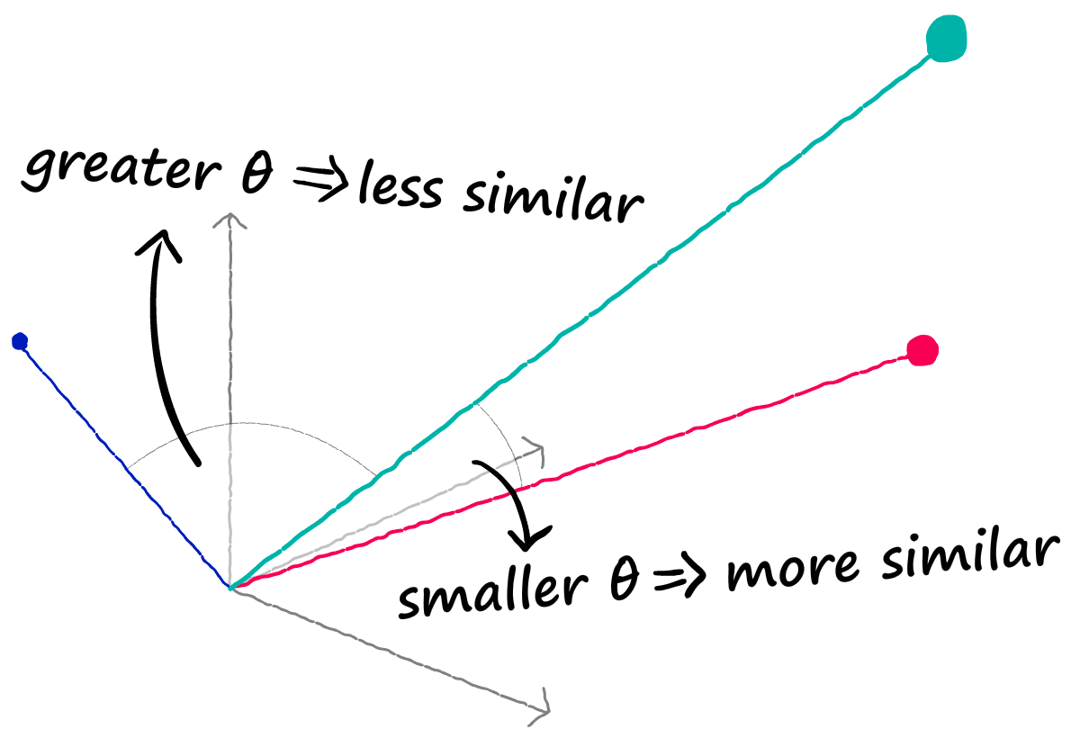
Now, with two correctly encoded dense vectors, we can use a similarity metric like Cosine similarity to calculate their semantic similarity. Vectors that are more aligned are more semantically alike, and vise-versa.

A smaller angle between vectors (calculated with cosine similarity) means they are more aligned. For dense vectors, this correlates to greater semantic similarity.

But there’s one problem, each sequence is represented by 512 vectors — not one vector.

So, this is where another — brilliant — adaption of BERT comes into play. Sentence-BERT allows us to create a single vector that represents our full sequence, otherwise known as a sentence vector [2].

We have two ways of implementing SBERT — the easy way using the sentence-tranformers library, or the slightly less easy way using transformers and PyTorch.

We’ll cover both, starting with the transformers with PyTorch approach so that we can get an intuition for how these vectors are built.

If you’ve used the HF transformers library, the first few steps will look very familiar. We initialize our SBERT model and tokenizer, tokenize our text, and process our tokens through the model.

a = "purple is the best city in the forest"
b = "there is an art to getting your way and throwing bananas on to the street is not it"  # this is very similar to 'g'
c = "it is not often you find soggy bananas on the street"
d = "green should have smelled more tranquil but somehow it just tasted rotten"
e = "joyce enjoyed eating pancakes with ketchup"
f = "as the asteroid hurtled toward earth becky was upset her dentist appointment had been canceled"
g = "to get your way you must not bombard the road with yellow fruit"  # this is very similar to 'b'

from transformers import AutoTokenizer, AutoModel
import torch

Initialize our HF transformer model and tokenizer - using a pretrained SBERT model.

tokenizer = AutoTokenizer.from_pretrained('sentence-transformers/bert-base-nli-mean-tokens')
model = AutoModel.from_pretrained('sentence-transformers/bert-base-nli-mean-tokens')

Tokenize all of our sentences.

tokens = tokenizer([a, b, c, d, e, f, g],
                          max_length=128,
                          truncation=True,
                          padding='max_length',
                          return_tensors='pt')

tokens.keys()

dict_keys(['input_ids', 'token_type_ids', 'attention_mask'])

tokens['input_ids'][0]

tensor([ 101, 6379, 2003, 1996, 2190, 2103, 1999, 1996, 3224,  102,    0,    0,
           0,    0,    0,    0,    0,    0,    0,    0,    0,    0,    0,    0,
           0,    0,    0,    0,    0,    0,    0,    0,    0,    0,    0,    0,
           0,    0,    0,    0,    0,    0,    0,    0,    0,    0,    0,    0,
           0,    0,    0,    0,    0,    0,    0,    0,    0,    0,    0,    0,
           0,    0,    0,    0,    0,    0,    0,    0,    0,    0,    0,    0,
           0,    0,    0,    0,    0,    0,    0,    0,    0,    0,    0,    0,
           0,    0,    0,    0,    0,    0,    0,    0,    0,    0,    0,    0,
           0,    0,    0,    0,    0,    0,    0,    0,    0,    0,    0,    0,
           0,    0,    0,    0,    0,    0,    0,    0,    0,    0,    0,    0,
           0,    0,    0,    0,    0,    0,    0,    0])

Process our tokenized tensors through the model.

outputs = model(**tokens)
outputs.keys()

odict_keys(['last_hidden_state', 'pooler_output'])

We’ve added a new sentence here, sentence g carries the same semantic meaning as b — without the same keywords. Due to the lack of shared words, all of our previous methods would struggle to find similarity between these two sequences — remember this for later.

Here we can see the final embedding layer, *last_hidden_state*.

embeddings = outputs.last_hidden_state
embeddings[0]

tensor([[-0.6239, -0.2058,  0.0411,  ...,  0.1490,  0.5681,  0.2381],
        [-0.3694, -0.1485,  0.3780,  ...,  0.4204,  0.5553,  0.1441],
        [-0.7221, -0.3813,  0.2031,  ...,  0.0761,  0.5162,  0.2813],
        ...,
        [-0.1894, -0.3711,  0.3034,  ...,  0.1536,  0.3265,  0.1376],
        [-0.2496, -0.5227,  0.2341,  ...,  0.3419,  0.3164,  0.0256],
        [-0.3311, -0.4430,  0.3492,  ...,  0.3655,  0.2910,  0.0728]],
       grad_fn=<SelectBackward>)

embeddings[0].shape

torch.Size([128, 768])

We have our vectors of length 768 — but these are not sentence vectors as we have a vector representation for each token in our sequence (128 here as we are using SBERT — for BERT-base this is 512). We need to perform a mean pooling operation to create the sentence vector.

The first thing we do is multiply each value in our embeddings tensor by its respective attention_mask value. The attention_mask contains ones where we have ‘real tokens’ (eg not padding tokens), and zeros elsewhere — this operation allows us to ignore non-real tokens.

mask = tokens['attention_mask'].unsqueeze(-1).expand(embeddings.size()).float()
mask.shape

torch.Size([7, 128, 768])

mask[0]

tensor([[1., 1., 1.,  ..., 1., 1., 1.],
        [1., 1., 1.,  ..., 1., 1., 1.],
        [1., 1., 1.,  ..., 1., 1., 1.],
        ...,
        [0., 0., 0.,  ..., 0., 0., 0.],
        [0., 0., 0.,  ..., 0., 0., 0.],
        [0., 0., 0.,  ..., 0., 0., 0.]])

Now we have a masking array that has an equal shape to our output `embeddings` - we multiply those together to apply the masking operation on our outputs.

masked_embeddings = embeddings * mask
masked_embeddings[0]

tensor([[-0.6239, -0.2058,  0.0411,  ...,  0.1490,  0.5681,  0.2381],
        [-0.3694, -0.1485,  0.3780,  ...,  0.4204,  0.5553,  0.1441],
        [-0.7221, -0.3813,  0.2031,  ...,  0.0761,  0.5162,  0.2813],
        ...,
        [-0.0000, -0.0000,  0.0000,  ...,  0.0000,  0.0000,  0.0000],
        [-0.0000, -0.0000,  0.0000,  ...,  0.0000,  0.0000,  0.0000],
        [-0.0000, -0.0000,  0.0000,  ...,  0.0000,  0.0000,  0.0000]],
       grad_fn=<SelectBackward>)

Sum the remaining embeddings along axis 1 to get a total value in each of our 768 values.

summed = torch.sum(masked_embeddings, 1)
summed.shape

torch.Size([7, 768])

Next, we count the number of values that should be given attention in each position of the tensor (+1 for real tokens, +0 for non-real).

counted = torch.clamp(mask.sum(1), min=1e-9)
counted.shape

torch.Size([7, 768])

Finally, we get our mean-pooled values as the `summed` embeddings divided by the number of values that should be given attention, `counted`.

mean_pooled = summed / counted
mean_pooled.shape

torch.Size([7, 768])

And those are our sentence vectors, using those we can measure similarity by calculating the cosine similarity between each.

from sklearn.metrics.pairwise import cosine_similarity
import numpy as np

# convert to numpy array from torch tensor
mean_pooled = mean_pooled.detach().numpy()

# calculate similarities (will store in array)
scores = np.zeros((mean_pooled.shape[0], mean_pooled.shape[0]))
for i in range(mean_pooled.shape[0]):
    scores[i, :] = cosine_similarity(
        [mean_pooled[i]],
        mean_pooled
    )[0]

scores

array([[ 1.00000012,  0.1869276 ,  0.2829769 ,  0.29628235,  0.2745102 ,
         0.10176259,  0.21696258],
       [ 0.1869276 ,  1.        ,  0.72058779,  0.51428956,  0.1174964 ,
         0.19306925,  0.66182363],
       [ 0.2829769 ,  0.72058779,  1.00000024,  0.4886443 ,  0.23568943,
         0.17157131,  0.55993092],
       [ 0.29628235,  0.51428956,  0.4886443 ,  0.99999988,  0.26985496,
         0.37889433,  0.52388811],
       [ 0.2745102 ,  0.1174964 ,  0.23568943,  0.26985496,  0.99999988,
         0.23422126, -0.01599787],
       [ 0.10176259,  0.19306925,  0.17157131,  0.37889433,  0.23422126,
         1.00000012,  0.22319663],
       [ 0.21696258,  0.66182363,  0.55993092,  0.52388811, -0.01599787,
         0.22319663,  1.        ]])

If we visualize our array, we can easily identify higher similarity sentences:

Heatmap showing cosine similarity between our SBERT sentence vectors — the score between sentences b and g is circled.

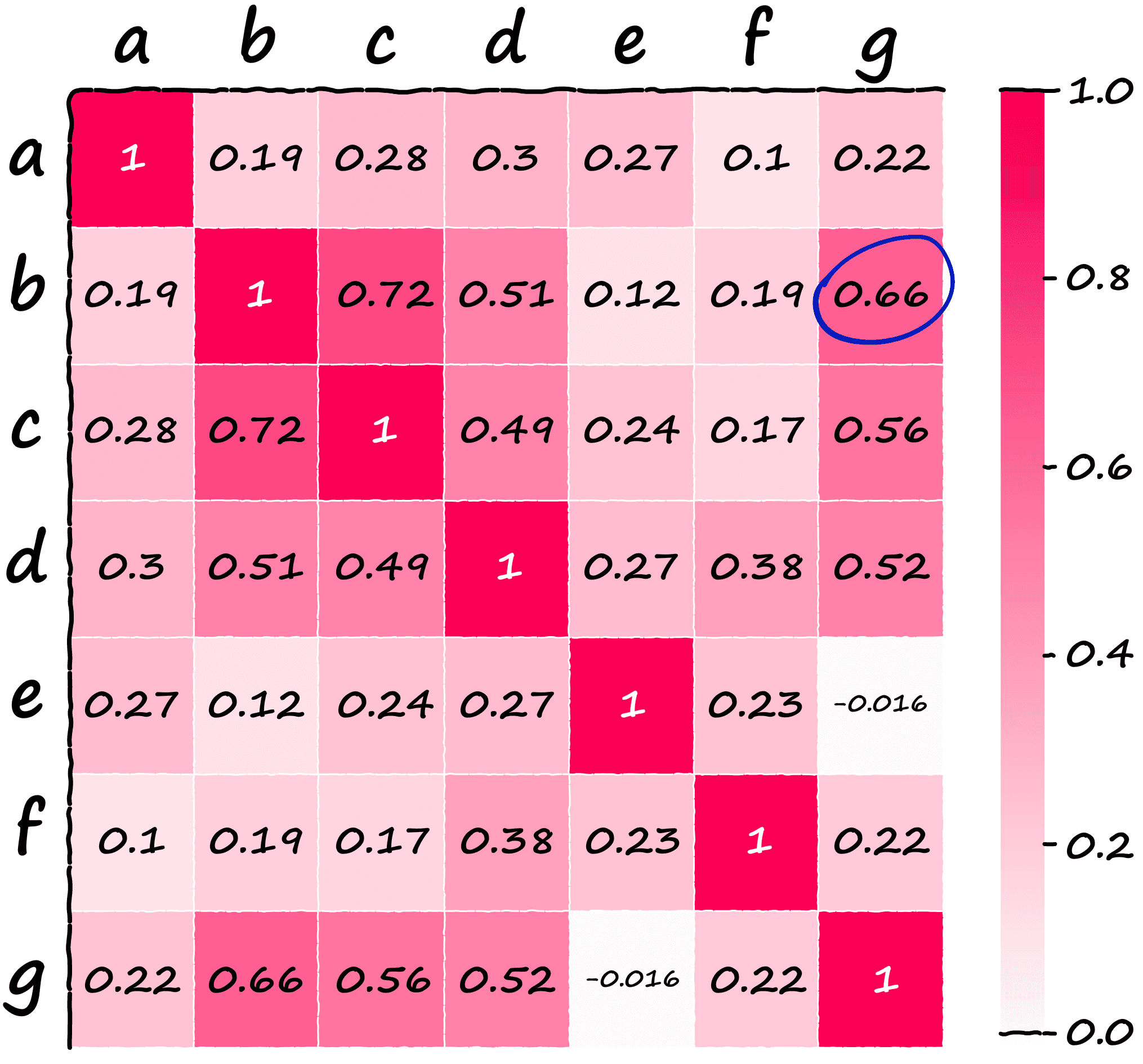
Now, think back to the earlier note about sentences b and g having essentially identical meaning whilst not sharing any of the same keywords.

We’d hope SBERT and its superior semantic representations of language to identify these two sentences as similar — and lo-and-behold the similarity between both is our second-highest score at 0.66 (circled above).

Now, the alternative (easy) approach is to use sentence-transformers. To get the exact same output as we produced above we write:

from sentence_transformers import SentenceTransformer

model = SentenceTransformer('bert-base-nli-mean-tokens')

We encode the sentences (producing our mean-pooled sentence embeddings) like so:

sentence_embeddings = model.encode([a, b, c, d, e, f, g])

And calculate the cosine similarity just like before.

from sklearn.metrics.pairwise import cosine_similarity
import numpy as np

# calculate similarities (will store in array)
scores = np.zeros((sentence_embeddings.shape[0], sentence_embeddings.shape[0]))
for i in range(sentence_embeddings.shape[0]):
    scores[i, :] = cosine_similarity(
        [sentence_embeddings[i]],
        sentence_embeddings
    )[0]

scores

array([[ 1.        ,  0.18692753,  0.28297687,  0.29628229,  0.27451015,
         0.1017626 ,  0.21696255],
       [ 0.18692753,  0.99999988,  0.72058773,  0.5142895 ,  0.11749639,
         0.19306931,  0.66182363],
       [ 0.28297687,  0.72058773,  1.00000024,  0.48864418,  0.2356894 ,
         0.17157122,  0.55993092],
       [ 0.29628229,  0.5142895 ,  0.48864418,  0.99999976,  0.26985493,
         0.3788943 ,  0.52388811],
       [ 0.27451015,  0.11749639,  0.2356894 ,  0.26985493,  0.99999982,
         0.23422126, -0.01599786],
       [ 0.1017626 ,  0.19306931,  0.17157122,  0.3788943 ,  0.23422126,
         1.00000012,  0.22319666],
       [ 0.21696255,  0.66182363,  0.55993092,  0.52388811, -0.01599786,
         0.22319666,  1.        ]])

Which, of course, is much easier.

That’s all for this walk through history with Jaccard, Levenshtein, and Bert!

We covered a total of six different techniques, starting with the straight-forward Jaccard similarity, w-shingling, and Levenshtein distance. Before moving onto search with sparse vectors — TF-IDF and BM25, and finishing up with state-of-the-art dense vector representations with SBERT.

References

[1] Market Capitalization of Alphabet (GOOG), Companies Market Cap

[2] N. Reimers, I. Gurevych, Sentence-BERT: Sentence Embeddings using Siamese BERT-Networks (2019), Proceedings of the 2019 Conference on Empirical Methods in 2019

Notebooks Repo

Runnable code notebooks: Jaccard, Levenshtein, TF-IDF, BM25, SBERT

*All images are by the author except where stated otherwise