Regularization in Neural Networks

Jun 30, 2023

Bala Priya C

Technical Writer

Neural networks can learn to represent complex relationships between network inputs and outputs. This representational power helps them perform better than traditional machine learning algorithms in computer vision and natural language processing tasks. However, one of the challenges associated with training neural networks is overfitting.

When a neural network overfits on the training dataset, it learns an overly complex representation that models the training dataset too well. As a result, it performs exceptionally well on the training dataset but generalizes poorly to unseen test data.

Regularization techniques help improve a neural network’s generalization ability by reducing overfitting. They do this by minimizing needless complexity and exposing the network to more diverse data. This article will cover common regularization techniques:

Early stopping
L1 and L2 regularization
Data augmentation
Addition of noise
Dropout

Let’s get started!

Early Stopping

Early stopping is one of the simplest and most intuitive regularization techniques. It involves stopping the training of the neural network at an earlier epoch; hence the name early stopping.

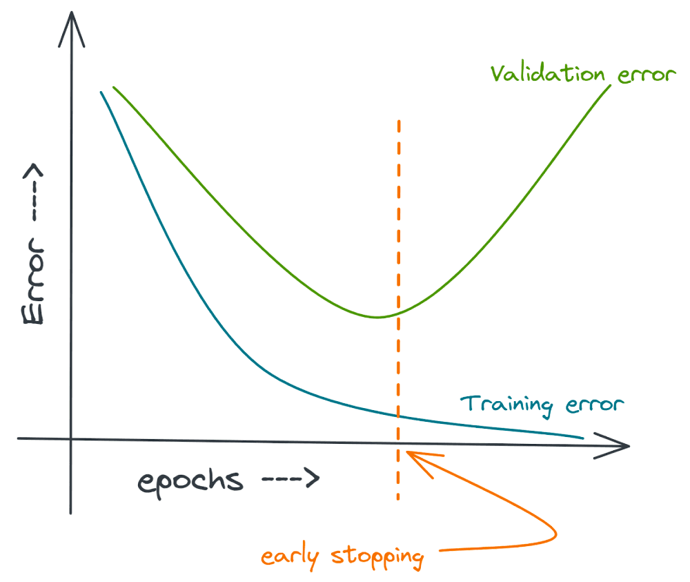
But how and when do we stop? As you train the neural network over many epochs, the training error decreases.

If the training error becomes too low and reaches arbitrarily close to zero, then the network is sure to overfit on the training dataset. Such a neural network is a high variance model that performs badly on test data that it has never seen before despite its near-perfect performance on the training samples.

Therefore, heuristically, if we can prevent the training loss from becoming arbitrarily low, the model is less likely to overfit on the training dataset, and will generalize better.

So how do we do it in practice? You can monitor one of the following:

The change in metrics such as validation error and validation accuracy
The change in the weight vector

Monitoring the Change in Validation Error

A simple approach is to monitor metrics such as validation error and validation accuracy as the neural network training proceeds, and use them to decide when to stop.

If we find that the validation error is not decreasing significantly or is increasing over a window of epochs, say p epochs, we can stop training. We can as well lower the learning rate and train for a few more epochs before stopping.

Error Change and Early Stopping

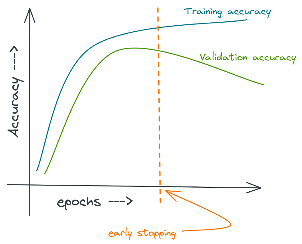
Equivalently, you can think in terms of the neural network’s accuracy on the training and validation datasets. Stopping early when the validation error starts increasing (or is no longer decreasing) is equivalent to stopping when the validation accuracy starts decreasing.

Monitoring the Validation Accuracy for Early Stopping

Monitoring the Change in the Weight Vector

Another way to know when to stop is to monitor the change in weights of the network. Let and denote the weight vectors at epochs and , respectively.

We can compute the L2 norm of the difference vector . We can stop training if this quantity is sufficiently small, say, less than .

Note: We’ll review Lp norms in greater detail in the section on L1 and L2 regularization. For now, you can think of the L2 norm as a non-negative quantity that captures the distance between any two vectors in a vector space.

But this approach of using the norm of the difference vector is not very reliable. Why? Certain weights might have changed a lot in the last k epochs, while some weights may have negligible changes. Therefore, the norm of the resultant difference vector can be small despite the drastic change in certain components of the weight vector.

A better approach is to compute the change in individual components of the weight vector. If the maximum change (across all components) is less than , we can conclude that the weights are not changing significantly, so we can stop the training of the neural network.

Data Augmentation

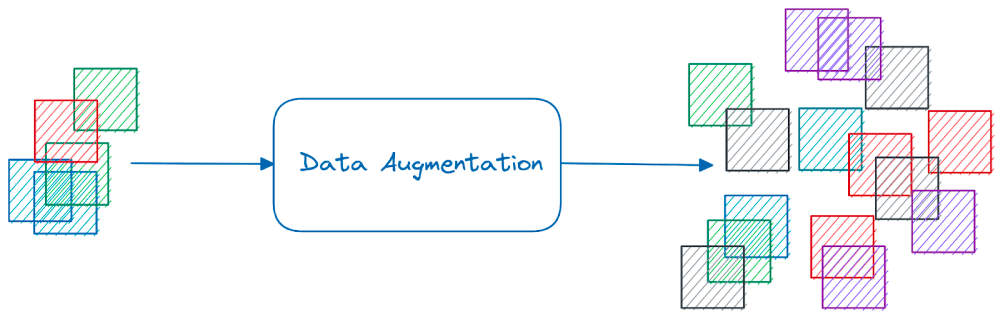
Data augmentation is a regularization technique that helps a neural network generalize better by exposing it to a more diverse set of training examples. As deep neural networks require a large training dataset, data augmentation is also helpful when we have insufficient data to train a neural network.

Let’s take the example of image data augmentation. Suppose we have a dataset with N training examples across C classes. We can apply certain transformations to these N images to construct a larger dataset.

Data Augmentation

What is a valid transformation? Any operation that does not alter the original label is a valid transformation. For example, a panda is a panda–whether it’s facing right or left, located near the center of the image or one of the corners.

In summary: we can apply any label-invariant transformation to perform data augmentation [1]. The following are some examples:

Color space transformations such as change of pixel intensities
Rotation and mirroring
Noise injection, distortion, and blurring

Newer Approaches to Image Data Augmentation

In addition to the basic color space and geometric image transformations, there are newer image augmentation techniques.

Mixup is a regularization technique that uses a convex combination of existing inputs to augment the dataset [2].

Suppose and are input samples belonging to the classes i and j, respectively; and are the one-hot vectors corresponding to the class labels i and j, respectively. A new image is formed by taking a convex combination of and :

A few other approaches to data augmentation include Cutout, CutMix, and AugMix. Cutout involves the random removal of portions of an input image during training [3]. CutMix replaces the removed sections with parts of another image [4].

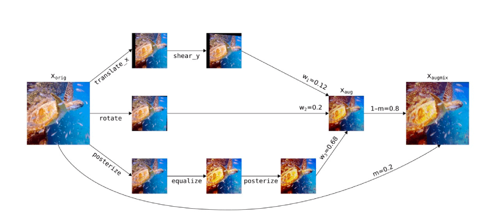
AugMix is a regularization technique that makes a neural network robust to distribution change [5]. Unlike mixup that uses images from two different classes, AugMix performs a series of transformations on the same image, and then uses a composition of these transformed images to get the resultant image.

How AugMix Works

L1 and L2 Regularization

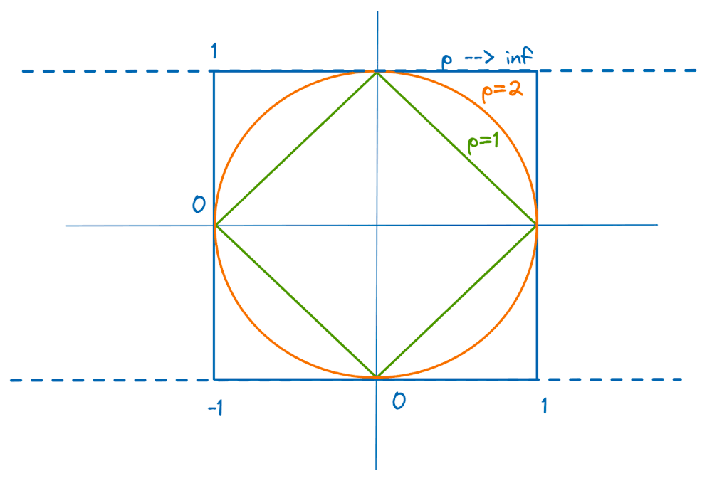
In general, Lp norms (for p>=1) penalize larger weights. They force the norm of the weight vector to stay sufficiently small. The Lp norm of a vector in n-dimensional space is given by:

L1 norm: When p=1, we get L1 norm, the sum of the absolute values of the components in the vector:

L2 norm: When p=2, we get L2 norm, the Euclidean distance of the point from the origin in n-dimensional vector space:

We’ll focus on L1 and L2 regularization. The unit L1 and L2 norm balls in two-dimensional plane are shown:

Unit Lp Norm Balls in 2D space for p = 1, 2

How and Why Regularization Works

Let and be the loss functions without and with regularization, respectively. The regularized loss function is given by:

where, is the regularization constant. Suppose is a sufficiently large constant.

When the weights become too large, the second term increases. However, as the goal of optimization is to minimize the loss function, the weights should decrease.

In particular, the L1 regularization promotes sparsity by forcing weights to zero. But why? Let’s take the example of 2D space: the L1 norm ball is a rhombus, and the regularized loss function is minimized at one of the vertices of the rhombus (where one of the coordinates is zero).

L1 Regularization Promotes Sparsity

In n-dimensional space, the loss function is minimized at one of the vertices of an n-dimensional rhombohedron; all other coordinates are zero.

Similarly, the regularized loss function with L2 regularization (also called L2 weight decay) is given by:

As with L1 regularization, if the weights become too large, increases, and consequently, the second term in the above equation increases. However, as the objective is to minimize the loss function, the algorithm favors smaller weights.

Even though the above equation looks like an unconstrained optimization problem, there is a constraint on the norm of the weight vector in a particular layer.

Unlike L1 regularization that forces weights to zero, L2 regularization shrinks weights while ensuring that important components of the weight vector are larger than the others. For a detailed mathematical analysis of how the regularized weight vector is related to the weight vector without regularization, refer to [9].

Addition of Noise

Another regularization approach is the addition of noise. You can add noise to the input, the output labels, or the gradients of the neural network.

Adding Noise to Input Data

When using the sum of squares loss function, adding Gaussian noise to the inputs is equivalent to L2 regularization [6].

To understand this equivalence, let’s assume a simple network with input layer and weights:

Adding Noise to Inputs

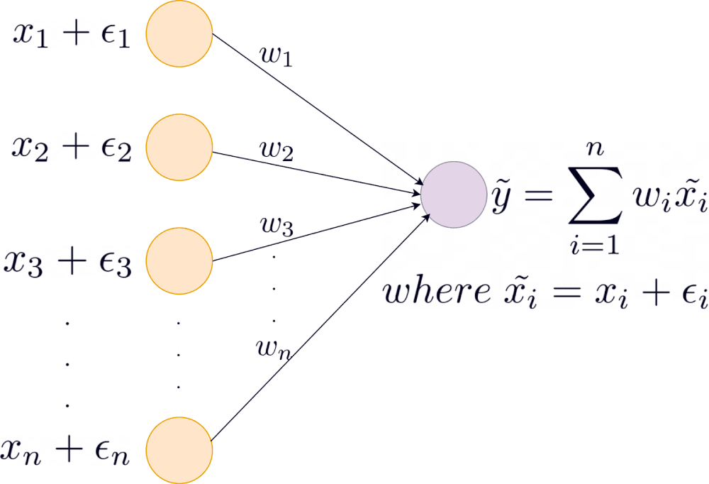
For each input sample , we add noise sampled from a normal distribution with zero mean and variance . The ’s are all independent. The output is given as follows:

Let denote the output in the absence of noise. Substituting the value of , we have:

If is the actual output, the expected sum of squares error is given by:

The second term in the above sum goes to zero as .

Using the independence of , terms in the summation that are of the form vanish: for all .
Further, as is a zero-mean random variable.

From the above equation, we see that the loss has the same form as L2 regularization.

Adding Noise to Output Labels

Adding noise to the output labels prevents the network from memorizing the training dataset by introducing perturbations in the output labels. Here are some techniques:

DisturbLabel

The DisturbLabel algorithm, proposed in [7], works as follows. Suppose there are N output classes: {1,2,3,…,N}. DisturbLabel works as follows:

Each training example is disturbed with the probability .
For each disturbed sample, the label is drawn from a uniform distribution over {1,2,3,…,N} irrespective of the true label.

Label Smoothing

Another approach to introducing noise in the output labels is using label smoothing. This regularization technique accounts for mislabeled samples in the training dataset.

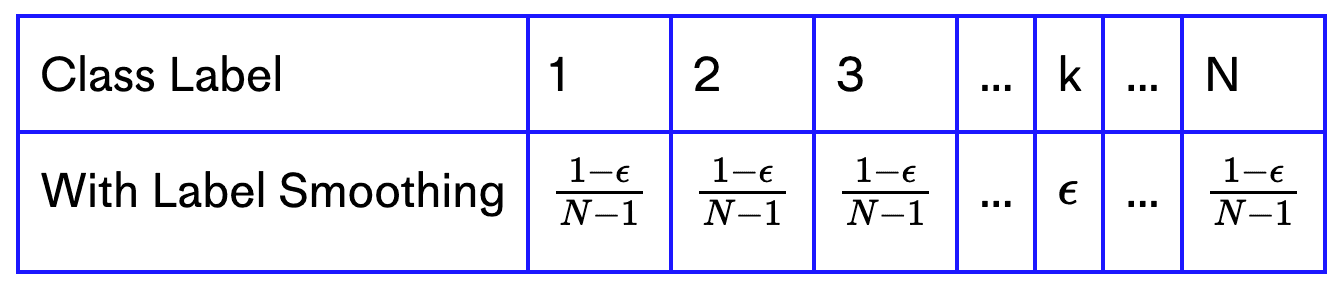
Suppose there are N total classes and the given label is k. In this case, the one-hot vector has 1 at the index corresponding to the class k and 0 elsewhere.

Class Label	1	2	3	...	k	...	N
Without Label Smoothing	0	0	0	...	1	...	0

When we perform label smoothing, we replace the hard target 1 with . To ensure the total probability is 1, we can set the other N-1 indices to .

Adding Noise to Gradients

If the gradient vector at step is , we update it by adding noise with zero mean and variance :

This updated gradient is used in backpropagation. Instead of fixed variance, [8] recommends the use of decaying variance (also called annealing Gaussian noise):

In [8], is chosen from the set {0.01, 0.3, 1.0} and is set to 0.55. Let us see how the variance varies with an increase in t. The variance of the noise added decreases as the training proceeds.

import pandas as pd
import matplotlib.pyplot as plt
import seaborn as sns

t = np.linspace(1,100)
y = np.zeros((len(t),3))
eta = [0.01,0.3,1]
gamma = 0.55

for idx,eta in enumerate(eta):
  y[:,idx] = eta/np.power(1+t,gamma)

df = pd.DataFrame({'t':t,
                   'η = 0.01': y[:,0],
                   'η = 0.3': y[:,1],
                   'η = 1': y[:,2]
                   })

df = df.melt('t',var_name="η values",value_name="noise variance")

sns.lineplot(data=df,x="t",y="noise variance",hue="η values")
plt.title("Annealing Gaussian Noise")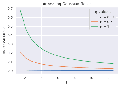

Dropout

Dropout is another popular regularization technique. To understand how dropout works, it’ll help to review the concept of model ensembling.

Revisiting Ensemble Methods

In traditional machine learning, model ensembling helps reduce overfitting and improve model performance. For a simple classification problem, we can take one of the following approaches:

Train multiple classifiers to solve the same task.
Train different instances of the same classifier for different subsets of the training dataset.

For a simple classification model, ensemble technique such as bagging involves training the same classifier—on different subsets of training data—sampled with replacement. Suppose there are N such instances. At test time, the test sample is run through each classifier, and an ensemble of their predictions is used.

In general, the performance of an ensemble is at least as good as the individual models; it cannot be worse than that of the individual models.

If we were to transpose this idea to neural networks, we could try doing the following (while identifying the limitations of this approach):

Train multiple neural networks with different architectures. Train a neural network on different subsets of the training data. However, training multiple neural networks is prohibitively expensive.
Even if we train N different neural networks, running the data point through each of the N models—at test time—introduces substantial computational overhead.

Dropout is a regularization technique that addresses both of the above concerns.

How Dropout Works

Let’s consider a simple neural network:

A Simple Neural Network

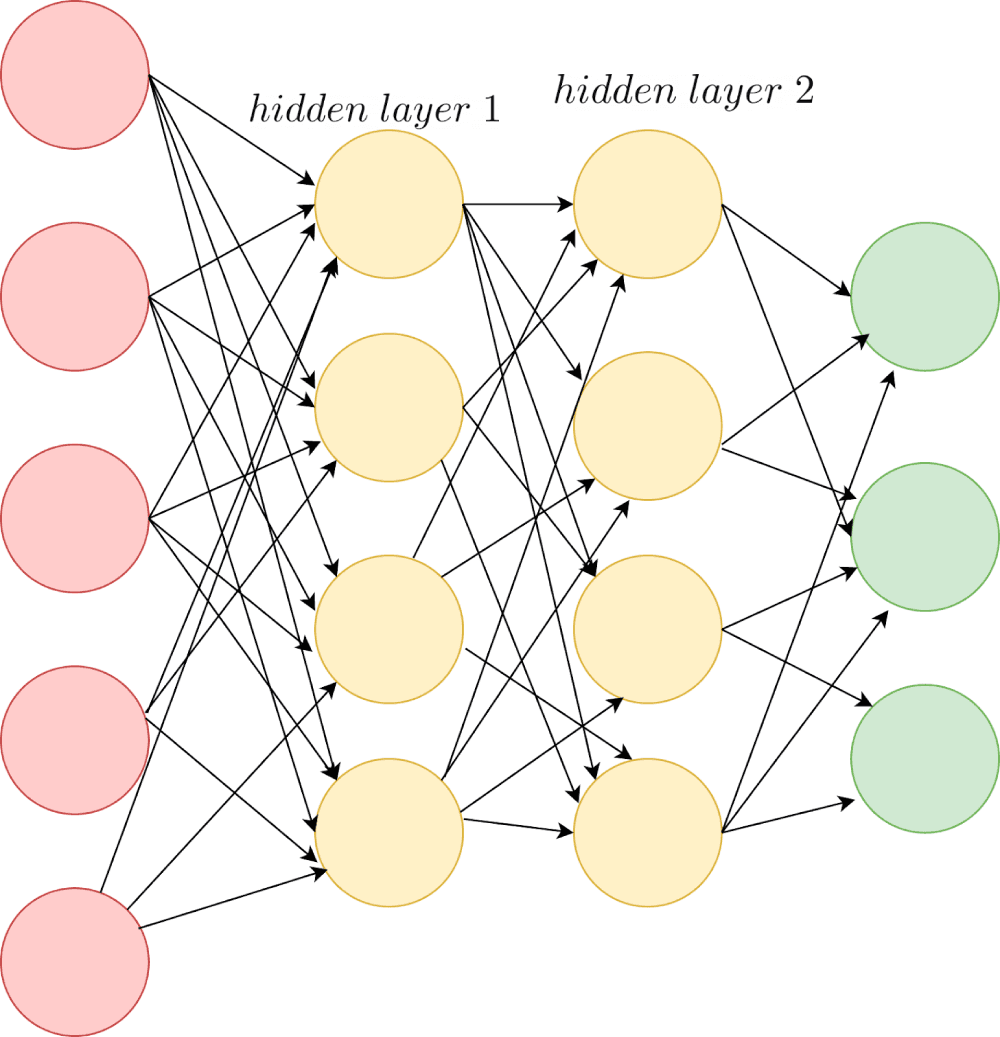
Dropout involves dropping neurons in the hidden layers and (optionally) the input layer. During training, each neuron is assigned a “dropout”probability, like 0.5.

With a dropout of 0.5, there’s a 50% chance of each neuron participating in training within each training batch. This results in a slightly different network architecture for each batch. It is equivalent to training different neural networks on different subsets of the training data.

Dropout

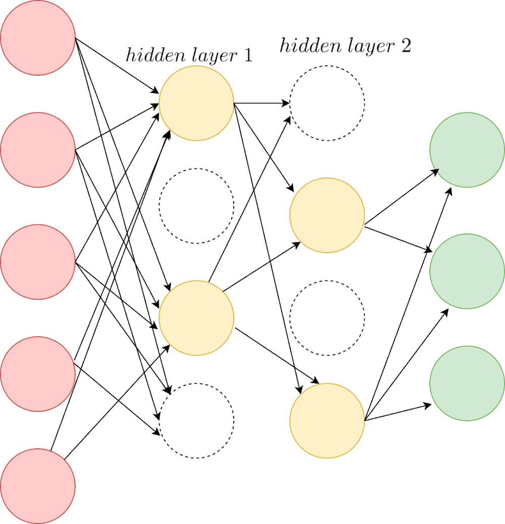
The weight matrix is initialized once at the beginning of the training. In general, for the k-th batch, backpropagation occurs only along those paths only through the neurons present for that batch. Meaning only the weights corresponding to neurons that are present get updates.

At test time, all the neurons are present in the network. So how do we account for the dropout during training? We weight each neuron’s output by the same probability p – proportional to the fraction of time the neuron was present during the training.

Summing Up

Regularization techniques aim to facilitate better generalization by minimizing complexity. To summarize the different techniques covered:

Early stopping reduces overfitting by stopping the training error from becoming too low consistently.
Data augmentation helps the model generalize better by exposing the model to diverse training examples during training. For image data, you can apply simple label-invariant transformations or newer techniques such as MixUp, AugMix, and CutMix.
In general, Lp norms penalize large weights. L1 regularization promotes sparsity by forcing many weights to go to zero. L2 regularization clips the weights from becoming too large while ensuring that the important components in the weight vector are larger than the other components.
We can add noise to the inputs, outputs, or gradients of the network to prevent a neural network from overfitting on the training data.
Dropout helps us emulate model ensembles by dropping out neurons during the training process with a fixed probability p, ensuring that a different neural network architecture is used for different batches during training. We weight a neuron’s output at test time by the same probability p.

In addition to these common regularization techniques, you can apply batch and layer normalization and use weight initialization techniques to improve the training of neural networks.

References

[1] R Wu et al., Deep Image: Scaling up Image Recognition, arXiv, 2015
[2] H. Zhang, M. Cisse, Y. N.Dauphin, D. Lopez-paz, Mixup: Beyond Empirical Risk Minimization, arXiv, 2017
[3] T. DeVries et al., Improved Regularization of Convolutional Neural networks with Cutout, arXiv, 2017
[4] S. Yun et al., CutMix: Regularization Strategy to Train Strong Classifiers with Localizable Features, ICCV 2019
[5] D. Hendryks, N. Mu et al., AugMix: A Simple Data Processing technique to improve Robustness and Uncertainty, ICLR 2020
[6] CM Bishop, Training with Noise is Equivalent to Tikhonov Regularization, Neural Computation, 1995
[7] L. Xie, J. Wang, Z.Wei, M. Wang, Q. Tian, DisturbLabel: Regularizing CNN on the Loss Layer (2016), CVPR 2016
[8] A. Neelakantan et al., Adding Gradient Noise Improves Learning for Very Deep Networks, arXiv, 2015
[9] Goodfellow et al., Deep learning, MIT Press, 2016
Was this article helpful?