Advanced Topic Modeling with BERTopic

Jun 23, 2023

Developer Advocate

90% of the world’s data is unstructured. It is built by humans, for humans. That’s great for human consumption, but it is very hard to organize when we begin dealing with the massive amounts of data abundant in today’s information age.

Organization is complicated because unstructured text data is not intended to be understood by machines, and having humans process this abundance of data is wildly expensive and very slow.

Fortunately, there is light at the end of the tunnel. More and more of this unstructured text is becoming accessible and understood by machines. We can now search text based on meaning, identify the sentiment of text, extract entities, and much more.

Transformers are behind much of this. These transformers are (unfortunately) not Michael Bay’s Autobots and Decepticons and (fortunately) not buzzing electrical boxes. Our NLP transformers lie somewhere in the middle, they’re not sentient Autobots (yet), but they can understand language in a way that existed only in sci-fi until a short few years ago.

Machines with a human-like comprehension of language are pretty helpful for organizing masses of unstructured text data. In machine learning, we refer to this task as topic modeling, the automatic clustering of data into particular topics.

BERTopic takes advantage of the superior language capabilities of these (not yet sentient) transformer models and uses some other ML magic like UMAP and HDBSCAN (more on these later) to produce what is one of the most advanced techniques in language topic modeling today.

BERTopic at a Glance

We will dive into the details behind BERTopic [1], but before we do, let us see how we can use it and take a first glance at its components.

To begin, we need a dataset. We can download the dataset from HuggingFace datasets with:

from datasets import load_dataset

data = load_dataset('jamescalam/python-reddit')

The dataset contains data extracted using the Reddit API from the /r/python subreddit. The code used for this (and all other examples) can be found here.

Reddit thread contents are found in the selftext feature. Some are empty or short, so we remove them with:

data = data.filter(
    lambda x: True if len(x['selftext']) > 30 else 0
)

We perform topic modeling using the BERTopic library. The “basic” approach requires just a few lines of code.

from bertopic import BERTopic
from sklearn.feature_extraction.text import CountVectorizer

# we add this to remove stopwords
vectorizer_model = CountVectorizer(ngram_range=(1, 2), stop_words="english")

model = BERTopic(
    vectorizer_model=vectorizer_model,
    language='english', calculate_probabilities=True,
    verbose=True
)
topics, probs = model.fit_transform(text)

From model.fit_transform we return two lists:

topics contains a one-to-one mapping of inputs to their modeled topic (or cluster).
probs contains a list of probabilities that an input belongs to their assigned topic.

We can then view the topics using get_topic_info.

In[5]:

freq = model.get_topic_info()
freq.head(10)

Out[5]:

   Topic  Count                                  Name
0     -1    196             -1_python_code_data_using
1      0     68          0_image_ampx200b_code_images
2      1     58    1_python_learning_programming_just
3      2     44         2_python_django_flask_library
4      3     32  3_link_title_thumbnail_datepublished
5      4     28            4_package_python_like_slap
6      5     27     5_spectra_space_asteroid_training
7      6     26    6_make_project ideas_ideas_comment
8      7     23                7_log_logging_use_conn
9      8     21    8_questions_thread_response_python

The top -1 topic is typically assumed to be irrelevant, and it usually contains stop words like “the”, “a”, and “and”. However, we removed stop words via the vectorizer_model argument, and so it shows us the “most generic” of topics like “Python”, “code”, and “data”.

The library has several built-in visualization methods like visualize_topics, visualize_hierarchy, and visualize_barchart.

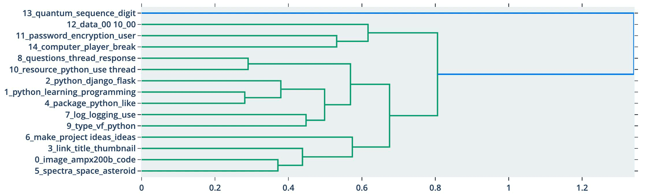
BERTopic’s visualize_hierarchy visualization allows us to view the “hierarchy” of topics.

These represent the surface level of the BERTopic library, which has excellent documentation, so we will not rehash that here. Instead, let’s try and understand how BERTopic works.

Overview

There are four key components used in BERTopic [2], those are:

A transformer embedding model
UMAP dimensionality reduction
HDBSCAN clustering
Cluster tagging using c-TF-IDF

We already did all of this in those few lines of BERTopic code; everything is just abstracted away. However, we can optimize the process by understanding the essentials of each component. This section will work through each component without BERTopic, and learn how they work before returning to BERTopic at the end.

Transformer Embedding

BERTopic supports several libraries for encoding our text to dense vector embeddings. If we build poor quality embeddings, nothing we do in the other steps will be able to help us, so it is very important that we choose a suitable embedding model from one of the supported libraries, which include:

Sentence Transformers
Flair
SpaCy
Gensim
USE (from TF Hub)

Of the above, the Sentence Transformers library provides the most extensive library of high-performing sentence embedding models. They can be found on HuggingFace Hub by searching for “sentence-transformers”.

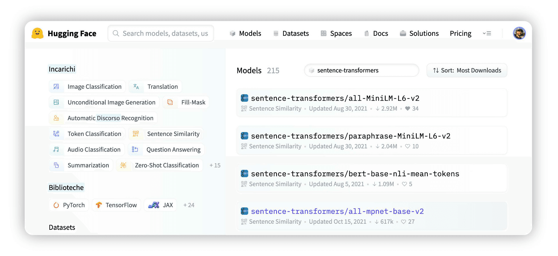
We can find official sentence transformer models by searching for “sentence-transformers” on HuggingFace Hub.

The first result of this search is sentence-transformers/all-MiniLM-L6-v2, this is a popular high-performing model that creates 384-dimensional sentence embeddings.

To initialize the model and encode our Reddit topics data, we first pip install sentence-transformers and then write:

In[5]:

from sentence_transformers import SentenceTransformer

model = SentenceTransformer('all-MiniLM-L6-v2')
model

Out[5]:

SentenceTransformer(
  (0): Transformer({'max_seq_length': 256, 'do_lower_case': False}) with Transformer model: BertModel 
  (1): Pooling({'word_embedding_dimension': 384, 'pooling_mode_cls_token': False, 'pooling_mode_mean_tokens': True, 'pooling_mode_max_tokens': False, 'pooling_mode_mean_sqrt_len_tokens': False})
  (2): Normalize()
)

In[6]:

import numpy as np
from tqdm.auto import tqdm

batch_size = 16

embeds = np.zeros((n, model.get_sentence_embedding_dimension()))

for i in tqdm(range(0, n, batch_size)):
    i_end = min(i+batch_size, n)
    batch = data['selftext'][i:i_end]
    batch_embed = model.encode(batch)
    embeds[i:i_end,:] = batch_embed

Out[6]:

100%|██████████| 195/195 [08:51<00:00,  2.73s/it]

Here we have encoded our text in batches of 16. Each batch is added to the embeds array. Once we have all of the sentence embeddings in embeds we’re ready to move on to the next step.

Dimensionality Reduction

After building our embeddings, BERTopic compresses them into a lower-dimensional space. This means that our 384-dimensional vectors are transformed into two/three-dimensional vectors.

We can do this because 384 dimensions are a lot, and it is unlikely that we really need that many dimensions to represent our text [4]. Instead, we attempt to compress that information into two or three dimensions.

We do this so that the following HDBSCAN clustering step can be done more efficiently. Performing the clustering step with 384-dimensions would be desperately slow [5].

Another benefit is that we can visualize our data; this is incredibly helpful when assessing whether our data can be clustered. Visualization also helps when tuning the dimensionality reduction parameters.

To help us understand dimensionality reduction, we will start with a 3D representation of the world. You can find the code for this part here.

We can apply many dimensionality reduction techniques to this data; two of the most popular choices are PCA and t-SNE.

PCA works by preserving larger distances (using mean squared error). The result is that the global structure of data is usually preserved [6]. We can see that behavior above as each continent is grouped with its neighboring continent(s). When we have easily distinguishable clusters in datasets, this can be good, but it performs poorly for more nuanced data where local structures are important.

t-SNE is the opposite; it preserves local structures rather than global. This localized focus results from t-SNE building a graph, connecting all of the nearest points. These local structures can indirectly suggest the global structure, but they are not strongly captured.

PCA focuses on preserving dissimilarity whereas t-SNE focuses on preserving similarity.

Fortunately, we can capture the best of both using a lesser-known technique called Uniform Manifold Approximation and Production (UMAP).

We can apply UMAP in Python using the UMAP library, installed using pip install umap-learn. To map to a 3D or 2D space using the default UMAP parameters, all we write is:

import umap

fit = umap.UMAP(n_components=3)  # by default this is 2
u = fit.fit_transform(data)

The UMAP algorithm can be fine-tuned using several parameters. Still, the simplest and most effective tuning can be achieved with just the n_neighbors parameter.

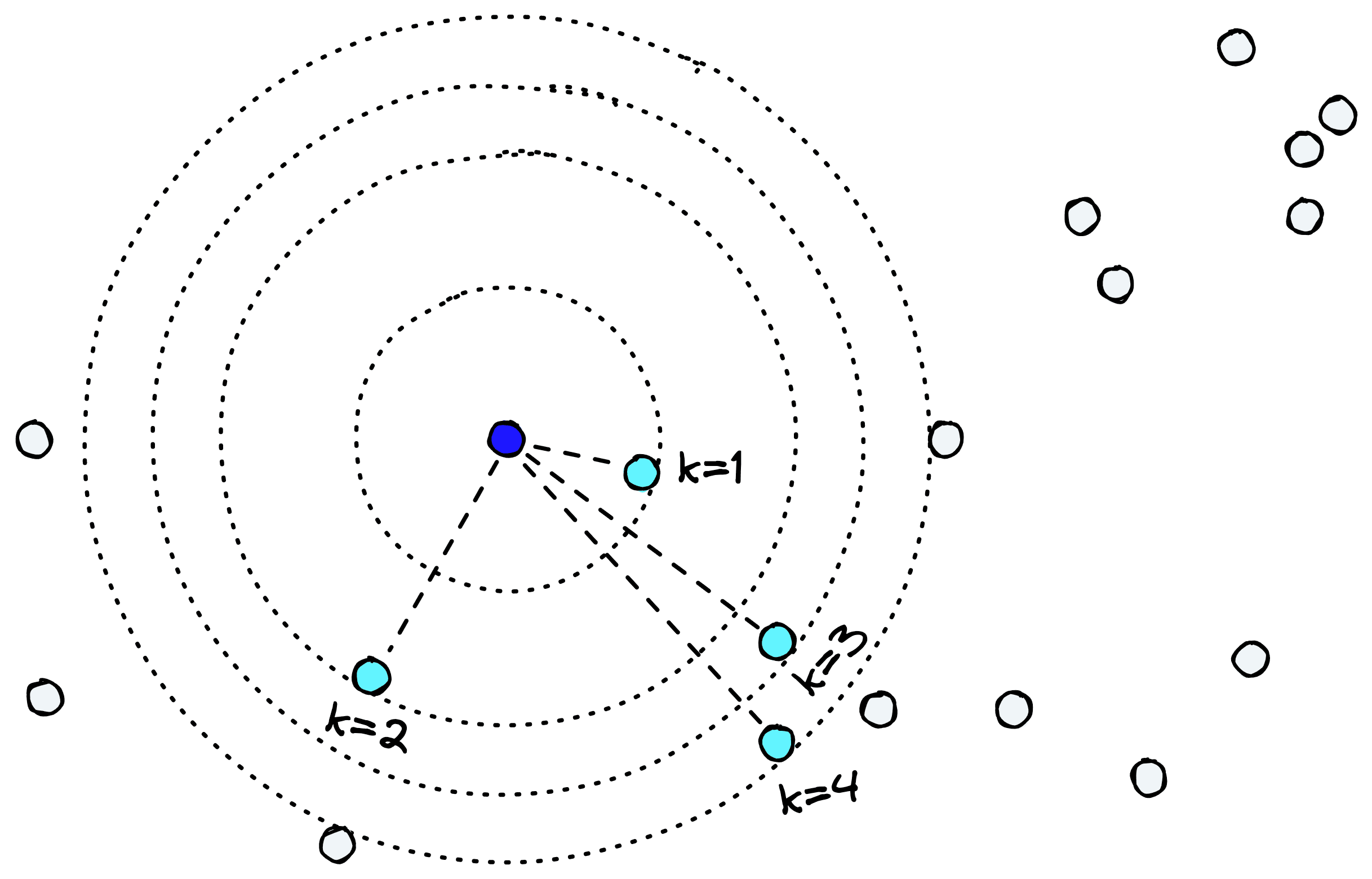
For each datapoint, UMAP searches through other points and identifies the kth nearest neighbors [3]. It is k, controlled by the n_neighbors parameter.

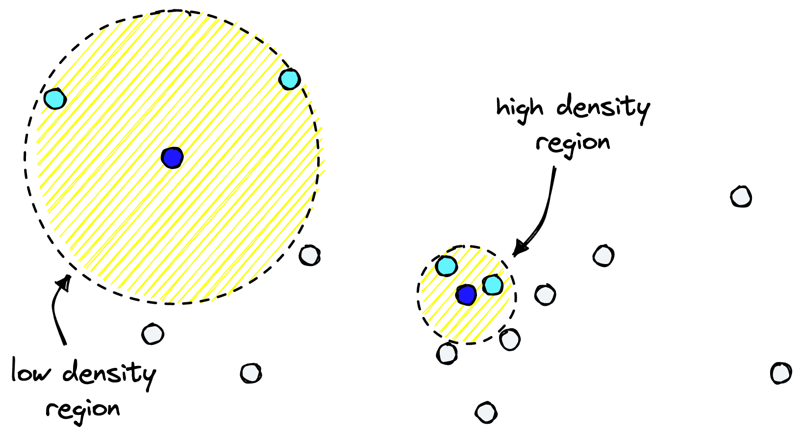
k and n_neighbors are synonymous here. As we increase n_neighbors the graph built by UMAP can consider more distant points and better represent the global structure.

Where we have many points (high-density regions), the distance between our point and its kth nearest neighbor is usually smaller. In low-density regions with fewer points, the distance will be much greater.

Density is measured indirectly using the distances between kth nearest neighbors in different regions.

UMAP will attempt to preserve distances to the kth nearest point is what UMAP attempts to preserve when shifting to a lower dimension.

By increasing n_neighbors we can preserve more global structures, whereas a lower n_neighbors better preserves local structures.

Higher n_neighbors (k) means we preserve larger distances and thus maintain more of the global structure.

Compared to other dimensionality reduction techniques like PCA or t-SNE, finding a good n_neighbors value allows us to preserve both local and global structures relatively well.

Applying it to our 3D globe, we can see neighboring countries remain neighbors. At the same time, continents are placed correctly (with North-South inverted), and islands are separated from continents. We even have what seems to be the Spanish Peninsula in “western Europe”.

UMAP maintains distinguishable features that are not preserved by PCA and a better global structure than t-SNE. This is a great overall example of where the benefit of UMAP lies.

UMAP can also be used as a supervised dimensionality reduction method by passing labels to the target argument if we have labeled data. It is possible to produce even more meaningful structures using this supervised approach.

With all that in mind, let us apply UMAP to our Reddit topics data. Using n_neighbors of 3-5 seems to work best. We can add min_dist=0.05 to allow UMAP to place points closer together (the default value is 1.0); this helps us separate the three similar topics from r/Python, r/LanguageTechnology, and r/pytorch.

fit = umap.UMAP(n_neighbors=3, n_components=3, min_dist=0.05)
u = fit.fit_transform(embeds)

With our data reduced to a lower-dimensional space and topics easily visually identifiable, we’re in an excellent spot to move on to clustering.

HDBSCAN Clustering

We have visualized the UMAP reduced data using the existing sub feature to color our clusters. It looks pretty, but we don’t usually perform topic modeling to label already labeled data. If we assume that we have no existing labels, our UMAP visual will look like this:

Now let us look at how HDBSCAN is used to cluster the (now) low-dimensional vectors.

Clustering methods can be broken into flat or hierarchical and centroid or density-based techniques [5]. Each of which has its own benefits and drawbacks.

Flat or hierarchical focuses simply on whether there is (or is not) a hierarchy in the clustering method. For example, we may (ideally) view our graph hierarchy as moving from continents to countries to cities. These methods allow us to view a given hierarchy and try to identify a logical “cut” along the tree.

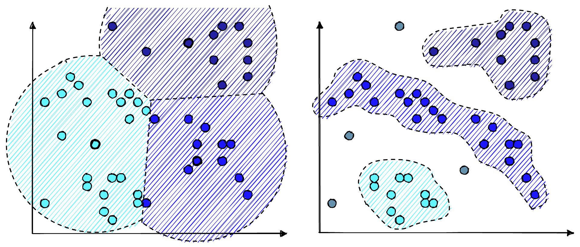
Hierarchical techniques begin from one large cluster and split this cluster into smaller and smaller parts and try to find the ideal number of clusters in the hierarchy.

The other split is between centroid-based or density-based clustering. That is clustering based on proximity to a centroid or clustering based on the density of points. Centroid-based clustering is ideal for “spherical” clusters, whereas density-based clustering can handle more irregular shapes and identify outliers.

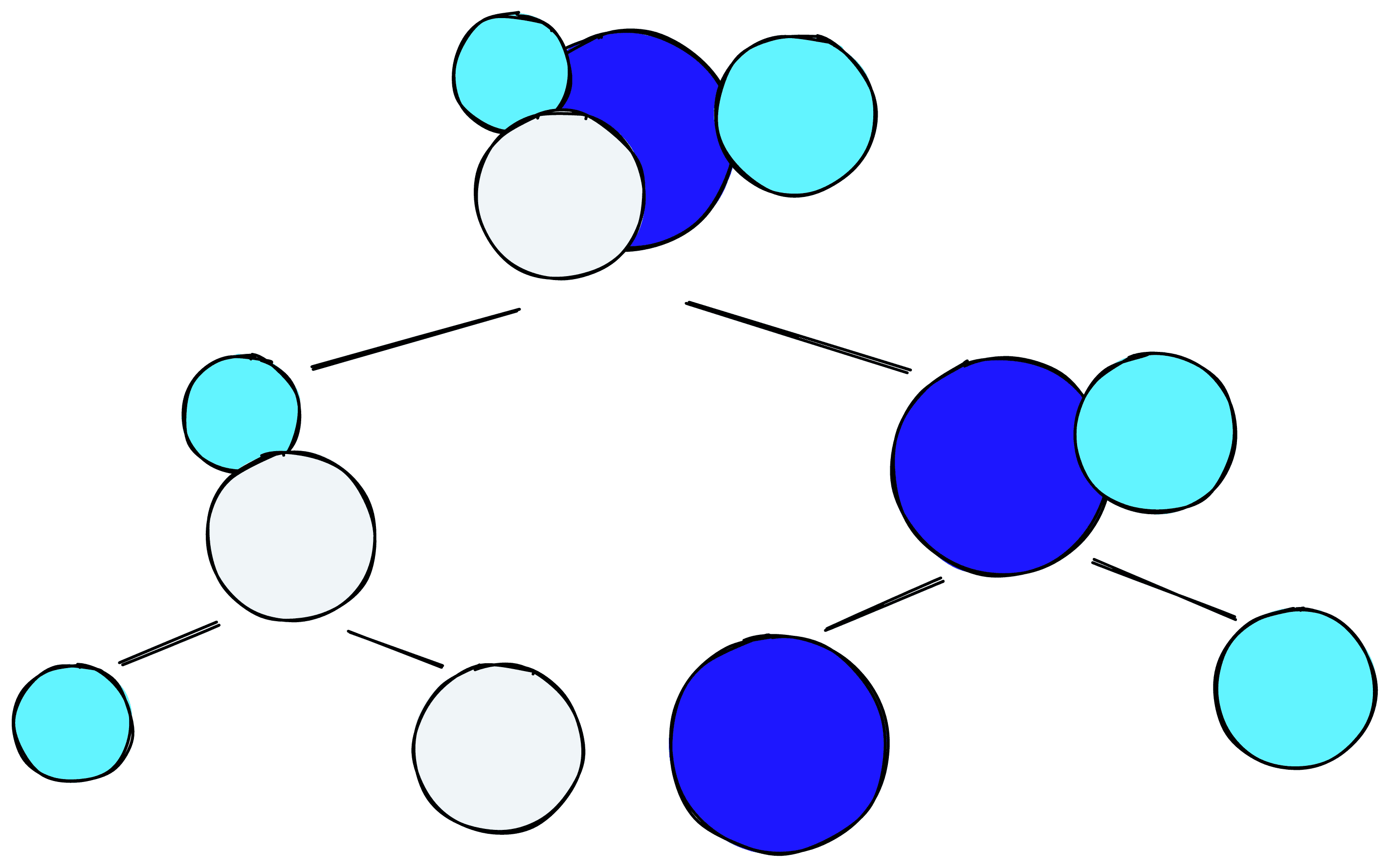
Centroid-based clustering (left) vs density-based clustering (right).

HDBSCAN is a hierarchical, density-based method. Meaning we can benefit from the easier tuning and visualization of hierarchical data, handle irregular cluster shapes, and identify outliers.

When we first apply HDBSCAN clustering to our data, we will return many tiny clusters, identified by the red circles in the condensed tree plot below.

In[22]:

import hdbscan

clusterer = hdbscan.HDBSCAN()
clusterer.fit(u)

Out[22]:

HDBSCAN()

In[23]:

clusterer.condensed_tree_.plot(select_clusters=True)

Out[23]:

<AxesSubplot:ylabel='$\\lambda$ value'>

Out[23]:

<Figure size 432x288 with 2 Axes>

The condensed tree plot shows the drop-off of points into outliers and the splitting of clusters as the algorithm scans by increasing lambda values.

HDBSCAN chooses the final clusters based on their size and persistence over varying lambda values. The tree’s thickest, most persistent “branches” are viewed as the most stable and, therefore, best candidates for clusters.

These clusters are not very useful because the default minimum number of points needed to “create” a cluster is just 5. Given our ~3K points dataset where we aim to produce ~4 subreddit clusters, this is small. Fortunately, we can increase this threshold using the min_cluster_size parameter.

In[28]:

clusterer = hdbscan.HDBSCAN(
    min_cluster_size=80)
clusterer.fit(u)

clusterer.condensed_tree_.plot(select_clusters=True)

Out[28]:

<AxesSubplot:ylabel='$\\lambda$ value'>

Out[28]:

<Figure size 432x288 with 2 Axes>

Better, but not quite there, we can try to reduce the min_cluster_size to 60 to pull in the three clusters below the green block.

In[29]:

clusterer = hdbscan.HDBSCAN(
    min_cluster_size=60)
clusterer.fit(u)

clusterer.condensed_tree_.plot(select_clusters=True)

Out[29]:

<AxesSubplot:ylabel='$\\lambda$ value'>

Out[29]:

<Figure size 432x288 with 2 Axes>

Unfortunately, this still pulls in the green block and even allows too small clusters (as on the left). Another option is to keep min_cluster_size=80 but add min_samples=40, to allow for more sparse core points.

In[30]:

clusterer = hdbscan.HDBSCAN(
    min_cluster_size=80, min_samples=40)
clusterer.fit(u)

clusterer.condensed_tree_.plot(select_clusters=True)

Out[30]:

<AxesSubplot:ylabel='$\\lambda$ value'>

Out[30]:

<Figure size 432x288 with 2 Axes>

Now we have four clusters, and we can visualize them using the data in clusterer.labels_.

A few outliers are marked in blue, some of which make sense (pinned daily discussion threads) and others that do not. However, overall, these clusters are very accurate. With that, we can try to identify the meaning of these clusters.

Topic Extraction with c-TF-IDF

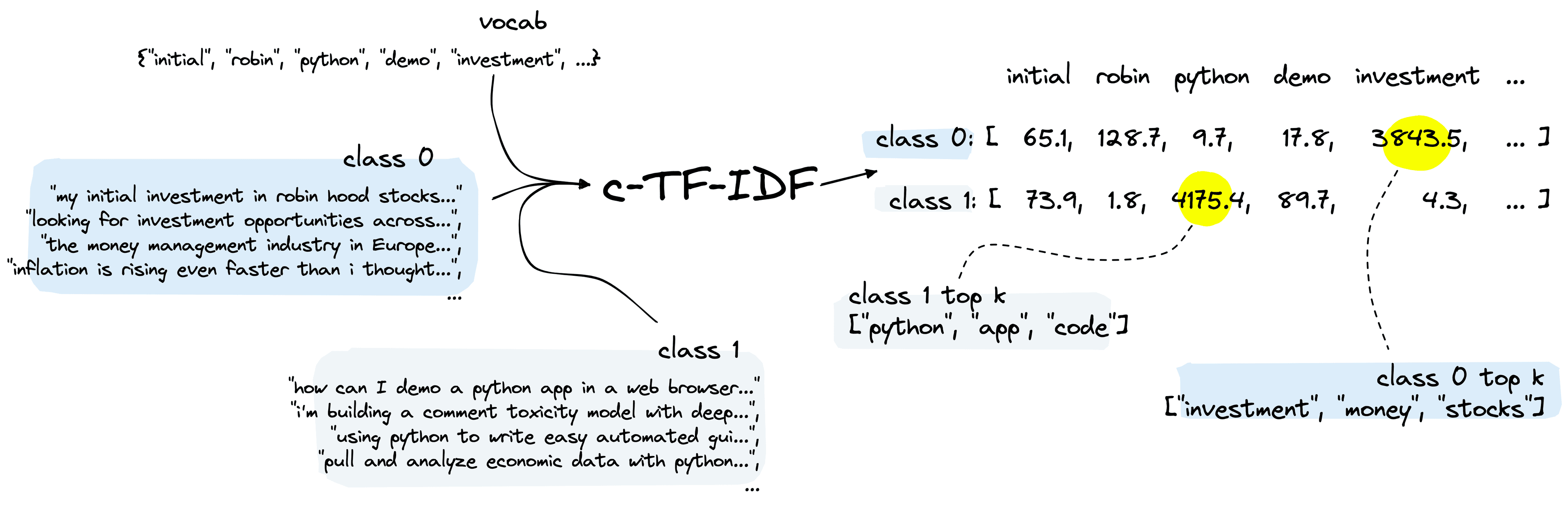
The final step in BERTopic is extracting topics for each of our clusters. To do this, BERTopic uses a modified version of TF-IDF called c-TF-IDF.

TF-IDF is a popular technique for identifying the most relevant “documents” given a term or set of terms. c-TF-IDF turns this on its head by finding the most relevant terms given all of the “documents” within a cluster.

c-TF-IDF looks at the most relevant terms from each class (cluster) to create topics.

In our Reddit topics dataset, we have been able to identify very distinct clusters. However, we still need to determine what these clusters talk about. We start by preprocessing the selftext to create tokens.

In[75]:

import re
import nltk

# first lowercase and remove punctuation
alpha = re.compile(r'[^a-zA-Z ]+')
data = data.map(lambda x: {
    'tokens': alpha.sub('', x['selftext']).lower()
})
# tokenize, separating by whitespace
data = data.map(lambda x: {
    'tokens': nltk.tokenize.wordpunct_tokenize(x['tokens'])
})
# remove stopwords
stopwords = set(nltk.corpus.stopwords.words('english'))
# stopwords from nltk are all lowercase (so are our tokens)
data = data.map(lambda x: {
    'tokens': word for word in x['tokens'] if word not in stopwords
})

Out[75]:

100%|██████████| 3118/3118 [00:00<00:00, 7893.81ex/s]

In[76]:

data[0]

Out[76]:

{'sub': 'investing',
 'title': 'Daily General Discussion and Advice Thread - March 03, 2022',
 'selftext': 'Have a general question?  Want to offer some commentary on markets?  Maybe... financial decisions!',
 'upvote_ratio': 0.84,
 'id': 't3_t5o82m',
 'created_utc': 1646301670.0,
 'class': -1,
 'tokens': ['have',
  'general',
  'question',
  'want',
  '...',
  'financial',
  'decisions']}

Part of c-TF-IDF requires calculating the frequency of term t in class c. For that, we need to see which tokens belong in each class. We first add the cluster/class labels to data.

# add the cluster labels to our dataset
data = data.add_column('class', clusterer.labels_)

Now create class-specific lists of tokens.

classes = {label: {'tokens': []} for label in set(clusterer.labels_)}
# add tokenized sentences to respective class
for row in data:
    classes[row['class']]['tokens'].extend(row['tokens'])

We can calculate Term Frequency (TF) per class.

In[80]:

tf = np.zeros((len(classes.keys()), len(vocab)))

for c, _class in enumerate(classes.keys()):
    for t, term in enumerate(tqdm(vocab)):
        tf[c, t] = classes[_class]['tokens'].count(term)

Out[80]:

100%|██████████| 31250/31250 [00:26<00:00, 1177.96it/s]
100%|██████████| 31250/31250 [00:15<00:00, 1979.75it/s]
100%|██████████| 31250/31250 [00:17<00:00, 1758.14it/s]
100%|██████████| 31250/31250 [00:10<00:00, 3052.47it/s]
100%|██████████| 31250/31250 [00:03<00:00, 8385.79it/s]

In[81]:

tf

Out[81]:

array([[  1.,   0.,   4., ...,   1., 177.,   1.],
       [  0.,   0.,  20., ...,   0.,  16.,   1.],
       [  0.,   1.,   4., ...,   0.,  51.,   5.],
       [  0.,   0.,   0., ...,   0.,  36.,   0.],
       [  0.,   0.,   0., ...,   0.,   0.,   0.]])

Note that this can take some time; our TF process prioritizes readability over any notion of efficiency. Once complete, we’re ready to calculate Inverse Document Frequency (IDF), which tells us how common a term is. Rare terms signify greater relevance than common terms (and will output a greater IDF score).

In[82]:

idf = np.zeros((1, len(vocab)))

# calculate average number of words per class
A = tf.sum() / tf.shape[0]

for t, term in enumerate(tqdm(vocab)):
    # frequency of term t across all classes
    f_t = tf[:,t].sum()
    # calculate IDF
    idf_score = np.log(1 + (A / f_t))
    idf[0, t] = idf_score

Out[82]:

100%|██████████| 31250/31250 [00:00<00:00, 215843.43it/s]

In[83]:

idf

Out[83]:

array([[10.65296781, 10.65296781,  7.32140112, ..., 10.65296781,
         5.0247495 ,  8.70719943]])

We now have TF and IDF scores for every term, and we can calculate the c-TF-IDF score by simply multiplying both.

In[84]:

tf_idf = tf*idf

In[85]:

tf_idf

Out[85]:

array([[ 10.65296781,   0.        ,  29.28560448, ...,  10.65296781,
        889.38066222,   8.70719943],
       [  0.        ,   0.        , 146.42802238, ...,   0.        ,
         80.39599207,   8.70719943],
       [  0.        ,  10.65296781,  29.28560448, ...,   0.        ,
        256.26222471,  43.53599715],
       [  0.        ,   0.        ,   0.        , ...,   0.        ,
        180.89098215,   0.        ],
       [  0.        ,   0.        ,   0.        , ...,   0.        ,
          0.        ,   0.        ]])

In tf_idf, we have a vocab sized list of TF-IDF scores for each class. We can use Numpy’s argpartition function to retrieve the index positions containing the greatest TF-IDF scores per class.

In[86]:

n = 5

In[87]:

top_idx = np.argpartition(tf_idf, -n)[:, -n:]
top_idx

Out[87]:

array([[31130,  7677, 15408, 24406, 24165],
       [ 1248, 15408,  4873, 17200, 27582],
       [29860, 10373, 17200,  2761,  1761],
       [21275, 21683, 15519,   802,  7088],
       [ 9974,  8792, 19143, 12105,  3664]])

Now we map those index positions back to the original words in the vocab.

In[88]:

vlist = list(vocab)

for c, _class in enumerate(classes.keys()):
    topn_idx = top_idx[c, :]
    topn_terms = [vlist[idx] for idx in topn_idx]
    print(topn_terms)

Out[88]:

['like', 'im', 'would', 'stock', 'market']
['data', 'would', 'nlp', 'model', 'text']
['training', 'pytorch', 'model', 'gt', 'x']
['using', 'project', 'use', 'code', 'python']
['useful', 'include', 'consider', 'financial', 'relevant']

Here we have the top five most relevant words for each cluster, each identifying the most relevant topics in each subreddit.

Back to BERTopic

We’ve covered a considerable amount, but can we apply what we have learned to the BERTopic library?

Fortunately, all we need are a few lines of code. As before, we initialize our custom embedding, UMAP, and HDBSCAN components.

from sentence_transformers import SentenceTransformer
from umap import UMAP
from hdbscan import HDBSCAN

embedding_model = SentenceTransformer('all-MiniLM-L6-v2')
umap_model = UMAP(n_neighbors=3, n_components=3, min_dist=0.05)
hdbscan_model = HDBSCAN(min_cluster_size=80, min_samples=40,
                        gen_min_span_tree=True,
                        prediction_data=True)

You might notice that we have added prediction_data=True as a new parameter to HDBSCAN. We need this to avoid an AttributeError when integrating our custom HDBSCAN step with BERTopic. Adding gen_min_span_tree adds another step to HDBSCAN that can improve the resultant clusters.

We must also initialize a vectorizer_model to handle stopword removal during the c-TF-IDF step. We will use the list of stopwords from NLTK but add a few more tokens that seem to pollute the results.

from sklearn.feature_extraction.text import CountVectorizer
from nltk.corpus import stopwords

stopwords = list(stopwords.words('english')) + ['http', 'https', 'amp', 'com']

# we add this to remove stopwords that can pollute topcs
vectorizer_model = CountVectorizer(ngram_range=(1, 2), stop_words=stopwords)

We’re now ready to pass all of these to a BERTopic instance and process our Reddit topics data.

from bertopic import BERTopic

model = BERTopic(
    umap_model=umap_model,
    hdbscan_model=hdbscan_model,
    embedding_model=embedding_model,
    vectorizer_model=vectorizer_model,
    top_n_words=5,
    language='english',
    calculate_probabilities=True,
    verbose=True
)
topics, probs = model.fit_transform(data['selftext'])

We can visualize the new topics with model.visualize_barchart()

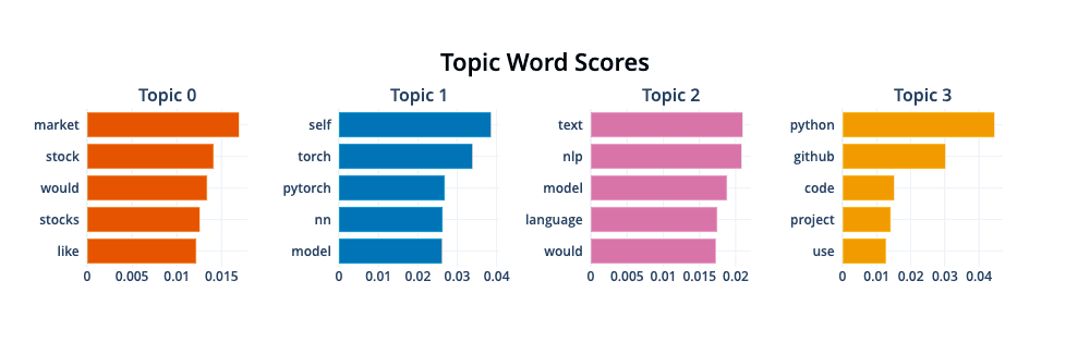
Our final topics produced using the BERTopic library with the tuned UMAP and HDBSCAN parameters.

We can see the topics align perfectly with r/investing, r/pytorch, r/LanguageTechnology, and r/Python.

Transformers, UMAP, HDBSCAN, and c-TF-IDF are clearly powerful components that have huge applications when working with unstructured text data. BERTopic has abstracted away much of the complexity of this stack, allowing us to apply these technologies with nothing more than a few lines of code.

Although BERTopic can be simple, you have seen that it is possible to dive quite deeply into the individual components. With a high-level understanding of those components, we can greatly improve our topic modeling performance.

We have covered the essentials here, but we genuinely are just scratching the surface of topic modeling in this article. There is much more to BERTopic and each component than we could ever hope to cover in a single article.

So go and apply what you have learned here, and remember that despite showing the incredible performance of BERTopic shown here, there is even more that it can do.