Streaming Embedding Generation with Databricks and Pinecone

Jun 30, 2023

Developer Advocate

Real-time data has become commonplace in many organizations, and with it, the ability to quickly process and store vector embeddings has become increasingly important. However, generating and storing these embeddings at scale in real-time scenarios can be challenging.

Real-time processing is challenging due to several reasons:

Data quality and consistency: Ensuring the quality of the data is crucial for accurate analysis and decision-making in real time environments.
Resource intensity: Large data volumes require significate resources and could incur sustainable cost, making efficient resource allocation critical.
Continuous data management: We need to constantly process and store incoming data. That means our system must be robust and resilient, regardless of what anomalies may exist in the data or how throughput may fluctuate.
Error sensitivity: Small errors can quickly propagate throughout the system, leading to inaccuracies that may impact the overall performance of the system
Technical complexity: Setting up and maintaining the necessary hardware and software for real-time pipelines can be intricate and challenging.

On top of all of these difficulties, adding vector embeddings to the pipeline makes the process even more complex and resource intensive.

Combining Databricks and Pinecone provides us with the perfect pipeline to answer these challenges. Databricks offers Structured streaming and Delta Live Tables as means to create a streaming pipeline. Pinecone provides the best solution for storing the embeddings produced in Databricks for consumption by downstream applications.

Architecture

Here’s a general overview of the pipeline’s architecture:

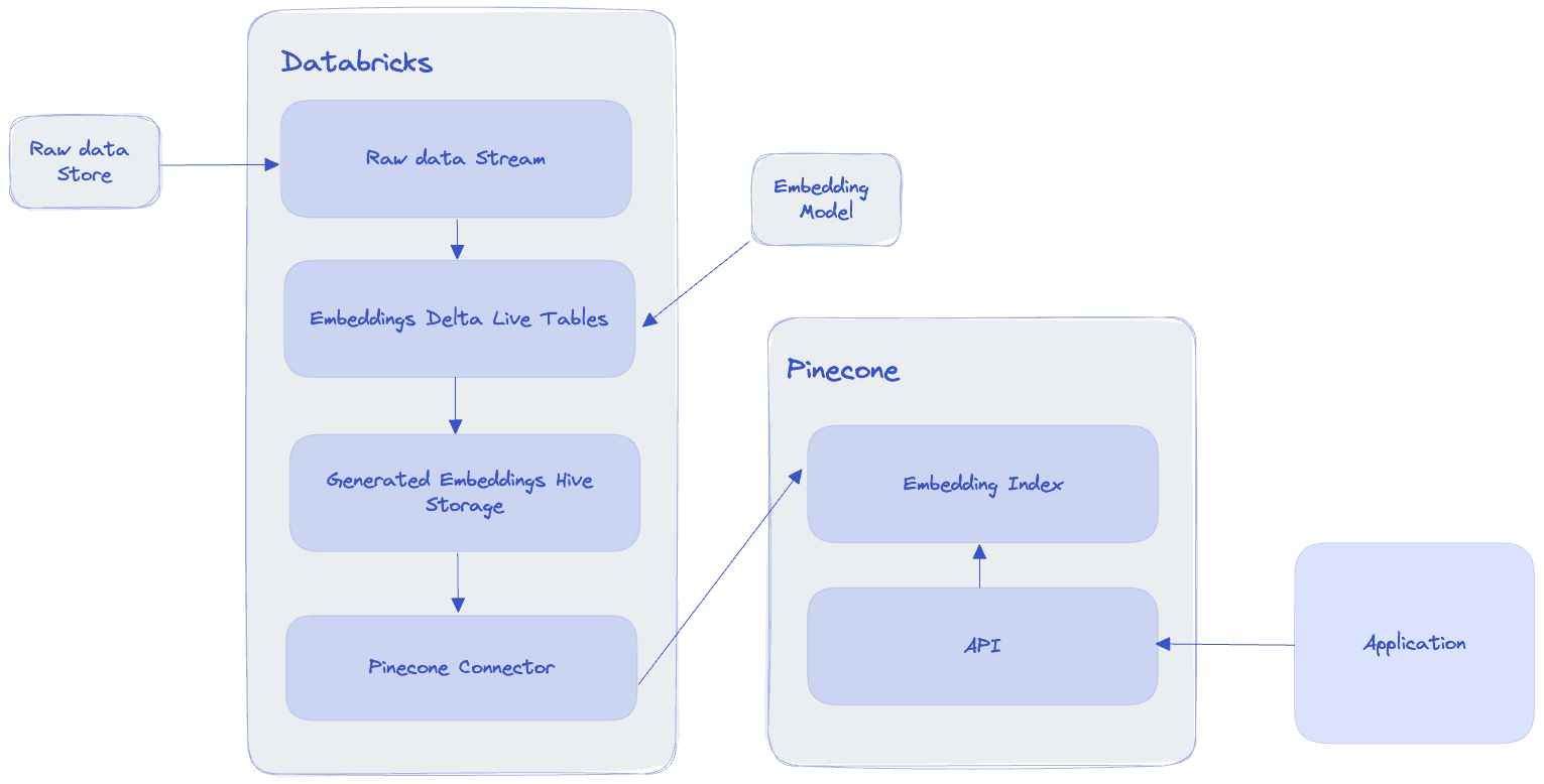
Databricks’s Delta lake architecture guides us to think of our data pipeline as having three tiers:

Bronze: Raw data ingestion - This tier is the initial stage where raw data is ingested into the system. It contains raw, unprocessed, and unfiltered data from various sources, including databases, logs, streams, and third-party APIs. Data in the Bronze tier is typically stored in its native format without any transformations.
Silver: Clean and enriched data - In the Silver tier, data is cleaned, processed, and enriched. Data quality issues, such as missing values, duplicates, and inconsistencies, are addressed. Data may also be enriched by adding additional attributes or combining datasets. The Silver tier usually contains data in a structured format, such as Parquet or Avro, optimized for analytics.
Gold: Aggregated and ready for consumption - The Gold tier contains data that has been further transformed and aggregated, making it ready for consumption by end-users, reports, machine learning models and other downstream applications.

In our pipeline, here’s how the tiers manifest:

The bronze layer includes the raw data from our store, which could be stored anywhere, for example an S3 bucket. In the example shown below, we use a Hive table to stand in place of this initial raw data.
The silver layer would include the steps to clean the data, split sentences and generate embeddings
The gold layer will be the final table where the generated embeddings are saved.

After the streaming process concludes, we pick it up with a separate job that will read the gold tier table and write it into Pinecone. From there, our downstream applications can interact with Pinecone via the Pinecone API to query the embeddings and modify them as needed.

Code

You can jump directly into the code or follow a step by step walkthrough below.

Install dependencies

To generate the embeddings, we’ll be using HuggingFace’s transformers. torch and senetencepiece are also dependencies that aren’t directly installed by transformers but are also required.

%pip install torch>=1.9.0
%pip install transformers>=4.15.0
%pip install sentencepiece

Import dependencies

We import dlt which allows us to decorate our functions with the @dlt decorator. This way, Databricks can pick up the functions and combine them in our Delta Live Tables pipeline.

import dlt
import pandas as pd
import numpy as np
from pyspark.sql.functions import *
from pyspark.sql.types import *
from typing import Iterator,Tuple
from transformers import AutoTokenizer, AutoModel

Bronze tier - reading the data

In this example, reading the data is straight forward - we simply consume a Hive table using the “delta” format. The “delta” format is the format used by Databricks’ Delta lakehouse.

# Read from our data source. This could be an S3 bucket, a Hive table etc.
@dlt.table
def raw_stream():
    return spark.readStream.format("delta").table("multi_news")

Silver tier - cleaning and preparing the data

Next, we add an “id” column with random uuids, and we drop the “summary” column that won’t be used for our embeddings. You can think of this as our “cleaning” step.

# Generate an ID for each document
@dlt.table
def documents():
    return (dlt.readStream("raw_stream").withColumn("id", expr("uuid()")).drop("summary"))

Our table includes a set of documents, which we want to break into sentences. We use the explode function to create a new column with the new split values. Then, we rename the old “id” column to “doc_id” and add a new “id” column with random values. This way, our sentences have a unique identifier, but also an identifier that ties them to the original document they came from.

# Read from "Document", split on ".", explode the table, rename the "id" column as doc_id and generate new IDs for each sentence
@dlt.table
def sentences():
    return (dlt.readStream("documents").withColumn("sentence", explode(split(col("document"), "\."))).withColumnRenamed("id", "doc_id")).withColumn("id", expr("uuid()"))

Gold tier - generating the embeddings

Next is where the heavy lifting happens: we define a Pandas UDF (User-Defined Function) to create embeddings for text data using a pre-trained Transformer model from the Hugging Face library. The UDF takes a Pandas DataFrame with sentences as input and outputs a DataFrame with the embeddings, namespace, and metadata for each sentence.

# Create the embeddings `
udf_result = StructType([
  StructField("id", StringType()),
  StructField("vector", ArrayType(FloatType())),
  StructField("namespace", StringType()),
  StructField("metadata", StringType())
])

@pandas_udf(udf_result, PandasUDFType.GROUPED_MAP)
def create_embeddings_with_transformers(pdf: pd.DataFrame)-> pd.DataFrame:
    # pdf is a pandas.DataFrame with one column "sentence"
    features = pdf.sentence
    tokenizer = AutoTokenizer.from_pretrained("sentence-transformers/all-MiniLM-L6-v2")
    model = AutoModel.from_pretrained("sentence-transformers/all-MiniLM-L6-v2")
    text = str(features)
    inputs = tokenizer(text, padding=True, truncation=True, return_tensors="pt", max_length=512)
    result = model(**inputs)
    embeddings = result.last_hidden_state[:, 0, :].cpu().detach().numpy()
    lst = embeddings.flatten().tolist()
    return pd.DataFrame({"id": pdf["id"].values, "vector": [lst], "namespace": "minilml6", "metadata": "{ \"original_doc\": \"" + pdf.doc_id + "\" }"})

Let’s break this down a bit:

udf_result defines the schema of the output DataFrame with four columns: id, vector, namespace, and metadata (using the StructType and StructField classes)
@pandas_udf(udf_result, PandasUDFType.GROUPED_MAP) is a decorator provided by PySpark to define a Pandas UDF with a specific output schema (udf_result) and UDF type (PandasUDFType.GROUPED_MAP). PandasUDFType.GROUPED_MAP is an enumeration value provided by PySpark to specify the type of a Pandas User-Defined Function (UDF). Pandas UDFs are a feature in PySpark that allows you to write UDFs using Python and pandas, leveraging the power and flexibility of pandas to process data within Spark DataFrames.
def create_embeddings_with_transformers(pdf: pd.DataFrame) -> pd.DataFrame: defines the UDF function that takes a pandas DataFrame pdf as input and returns a pandas DataFrame as output.
Inside the function, the features variable is assigned the values in the “sentence” column of the input DataFrame.
tokenizer and model are created using the Hugging Face library’s AutoTokenizer and AutoModel classes. They are initialized with a pre-trained Transformer model called “sentence-transformers/all-MiniLM-L6-v2”.
The text variable is created by converting the features (the sentences) to a string. If this conversion is not performed, we may encounter issues when passing the input data to the tokenizer, since it expects text data in the form of a string or a list of strings.
The inputs variable is created by tokenizing the text using the tokenizer. Padding, truncation, and max_length are set to ensure the input is in the correct format for the Transformer model.
The result variable is created by passing the inputs to the model. This step generates the embeddings for the input text.
The embeddings variable is created by extracting the last hidden state of the Transformer model’s output, which corresponds to the embeddings for the input text. The embeddings are then detached from the model’s computation graph and converted to a NumPy array.
The lst variable is created by flattening the embeddings array and converting it to a list.
The function returns a pandas DataFrame matching our schema. The id and vector columns contain the original id and embeddings for each sentence. The metadata column contains a JSON string with the doc_id of the original document.

Next, we simply create a table that will run this UDF and store its results.

@dlt.create_table(comment="extract text embeddings",
                  schema= """
                  id STRING,
                  vector ARRAY<FLOAT>,
                  namespace STRING,
                  metadata STRING
                  """)
def embeddings():
    return (dlt.readStream("sentences").groupby("id").apply(create_embeddings_with_transformers))

Running the pipeline

To start the DLT pipeline, we’ll need to first set it up. In the “Workflows” tab, navigate to the “Delta Live Tables” tab and click “Create pipeline from an existing notebook”.

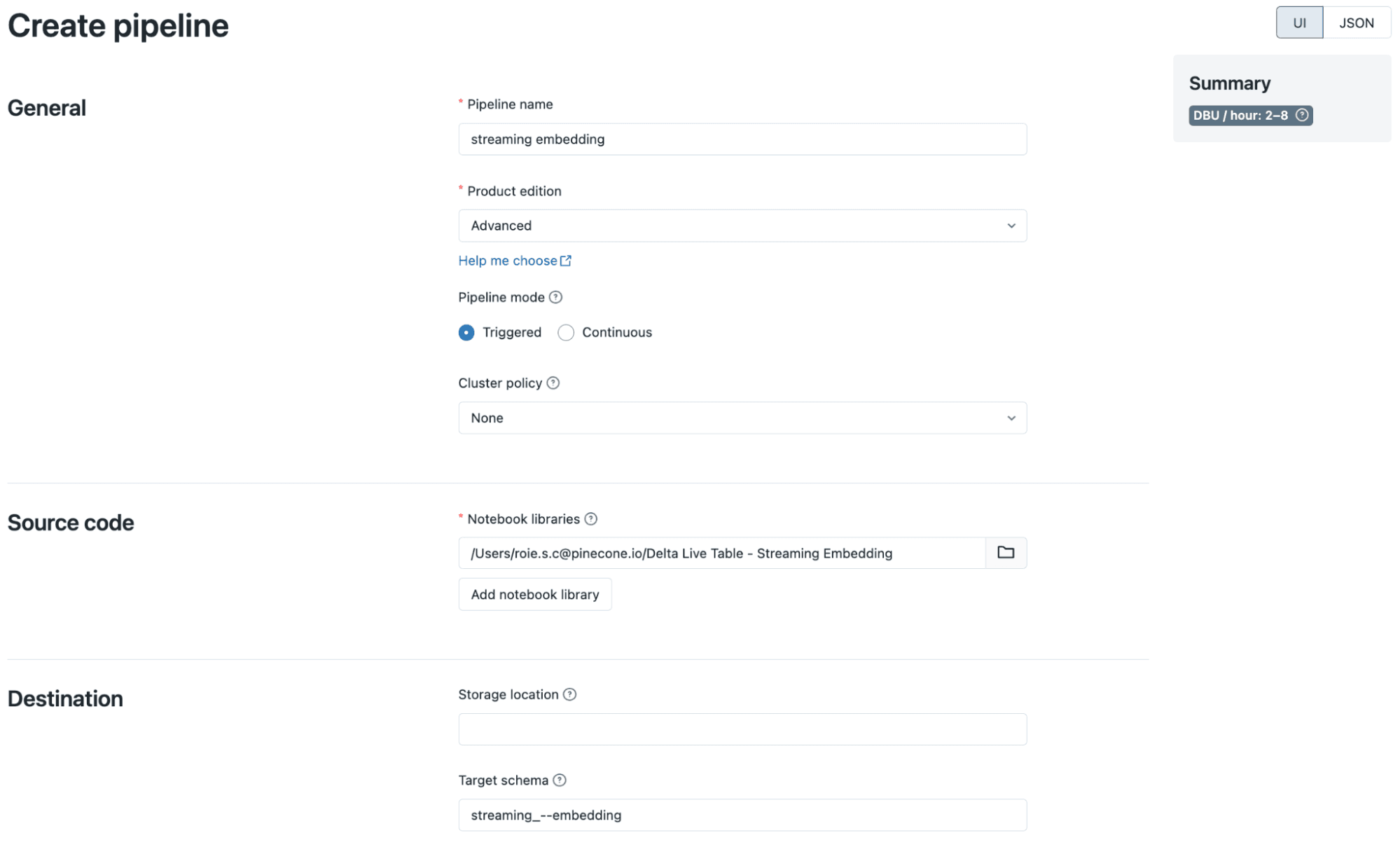
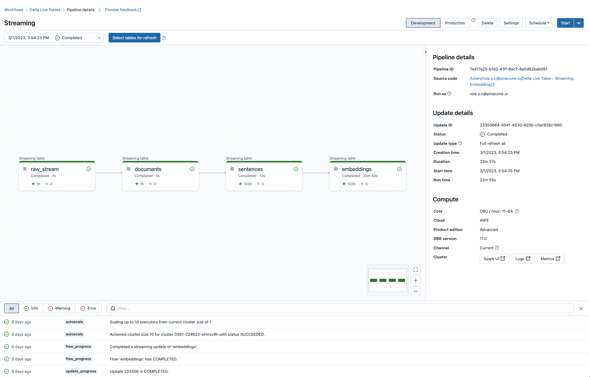
You’ll then be able to run the pipeline and inspect the execution of each step.

Writing the embeddings to Pinecone

After we are done with creating the embeddings, we’ll write them to Pinecone. Due to the current limitation on Delta Lake, Maven dependencies can’t be added to the pipeline, which is why we’ll use a scheduled job instead of another step in the DLT pipeline.

You can follow the instructions for setting up the cluster for this job with the necessary dependencies, and then run the following to write the embeddings into Pinecone:

df = spark.read.table("streaming_embedding.embeddings")
df.write
 .option("pinecone.apiKey", "YOUR_PINECONE_API_KEY")
 .option("pinecone.environment", "YOUR_PINECONE_ENVIORNMENT")
 .option("pinecone.projectName", "YOUR_PINECONE_PROJECT_NAME")
 .option("pinecone.indexName", "YOUR_INDEX_NAME")
 .format("io.pinecone.spark.pinecone.Pinecone")
 .mode("append")
 .save()

Final Thoughts

In the context of real-time data processing for AI, Databricks and Pinecone provide a powerful and efficient solution for generating, processing, and storing vector embeddings at scale. The three-tier Delta lake architecture (Bronze, Silver, and Gold) provides a well-structured approach to data processing, ensures quality and consistency. Databricks Delta Live Tables and Structured Streaming work together to create a seamless and scalable pipeline for real-time data processing, while Pinecone enables downstream applications to easily query and manipulate those embeddings. The real-time processing approach is already being widely applied in the realms of big data, and now we’re seeing how it can connect with the world of AI.

Thank you to Nitin Wagh, Avinash Sooriyarachchi and Sathish Gangichetty from Databricks for their contributions to this post.

Share via: