This is a comparison of Approximate Nearest Neighbor (ANN) speeds between Pinecone and several flavors of Elasticsearch. Thanks to Dmitry Kan, whose article is referenced here, for reviewing drafts of this post and providing valuable suggestions.
Semantic search applications have two core ingredients: Text documents represented as vector embeddings that capture meaning, and a search algorithm to retrieve semantically similar items.
BERT is a popular word embedding model because its pretrained versions provide high-quality embeddings without any additional training. However, those embeddings are high-dimensional (768 in our experiment), making it unbearably slow to search with k-nearest-neighbor (KNN) algorithms.
Fortunately, there are ways to speed things up considerably. One article shows how to search through BERT (or any other) embeddings progressively faster in Elasticsearch, starting with native, then with the Elastiknn plugin, then with Approximate k-NN in Open Distro for Elasticsearch, and finally with a GSI Associative Processing Unit (APU).
In the end, the author accelerated a million-document search from 1,500ms with Elasticsearch to 93ms with the GSI APU. An improvement of 6.1x — not bad! Not to mention the reduced index sizes and indexing times.
We wanted to take this experiment even further. Using Pinecone vector search we improved search speeds by 2.4x compared to Elasticsearch with GSI APU, and by 4.4x compared to Open Distro for Elasticsearch. All while maintaining a rank@k recall of 0.991.
Here’s how we did it.
ANN and Vector Indexes
Pinecone uses approximate-nearest-neighbor (ANN) search instead of k-nearest-neighbor (kNN). ANN is a method of performing nearest neighbor search where we trade off some accuracy for a massive boost in performance. Instead of going through the entire list of objects and finding the exact neighbors, it retrieves a “good guess” of an object’s neighbors.
A vector index is a specialized data structure tailor-made for performing a nearest neighbor search (approximate or exact) on vectors. An index allows us to insert, fetch and query our vectors efficiently. Pinecone employs its search algorithm and index that scales up to billions of vectors with extremely high throughput.

The Setup
The environment is not too relevant since Pinecone is a distributed service and your query and index times depend on the network rather than the machine itself. Though a beefier notebook instance means less time to compute embeddings. I used a GCP Notebook instance (n1-standard-8 US-West) for this experiment.
We used the same dataset, model, and approach as the reference article, using Pinecone instead for performing the search. We used the DBpedia dataset containing full abstracts of Wikipedia articles and SBERT from SentenceTransformers for creating embeddings.
You can find code for pre-processing the data in the GitHub repository from the reference article. Since Pinecone is a managed service, we can create and work with an index using its python client directly from the notebook. The code is available publicly.
Once we have the embeddings ready, searching with Pinecone is a three-step process: Create the index, upsert the embeddings, and query the index.
Here are a few snippets from the code to see how we used Pinecone for this experiment.
!pip install --quiet -U pinecone-client

import pinecone
pinecone.init(api_key=api_key)

index_name = 'bert-stats-test'

pinecone.create_index(index_name,metric='cosine', shards=shards)

def upload_items(items_to_upload: List, batch_size: int) -> float:
    print(f"\nUpserting {len(items_to_upload)} vectors...")
    start = time.perf_counter()
    upsert_cursor = index.upsert(items=items_to_upload,batch_size=batch_size)
    end = time.perf_counter()
    return (end - start) / 60.0
The Test
Pinecone runs in the cloud and not on your local machine. We changed how we query from the original article to make the comparisons better. Since my instance was on GCP (and Pinecone on AWS), querying an index across the internet adds overhead like network, authentication, parsing, etc. To estimate the speeds better, we queried the index in two ways:
- Send 10 single queries and average the speed.
- Send 10 batched queries with batch size = 1000 and calculate the average.
With batched queries, we lower the overheads per query. One way to ensure lower latencies is deploying your application in the same region and cloud service provider as Pinecone. Currently, our production servers run on AWS in US-West, but we can deploy Pinecone in any region on AWS or GCP.
Batching queries also has other practical applications apart from improving per query latency. Most notably, when you have a set of queries that you know you want to make beforehand, it’s better to send them in a batch.
Here’s our query function:
def query(test_items: List, index):
    print(f"\nQuerying...")
    times = []
    #For single queries, we pick 10 queries
    for test_item in test_items[:10]:
        start = time.perf_counter()
        #test_item is an array of [id,vector]
        query_results = index.query(queries=[test_item[1]],disable_progress_bar=True) # querying vectors with top_k=10
        end = time.perf_counter()
        times.append((end-start))
    #For batch queries, we pick 1000 vectors at perform 10 queries
    print(f"\n Batch Querying...")
    batch_times = []
    for i in range(0,10000, 1000):
        start = time.perf_counter()
        batch_items = test_items[i:i+1000]
        vecs = [item[1] for item in batch_items]
        query_results = index.query(queries=vecs,disable_progress_bar=True)
        end = time.perf_counter()
        batch_times.append((end-start))
    return mean(times)*1000,mean(batch_times)*1000
Using the setup and query method above, we saw the following results:
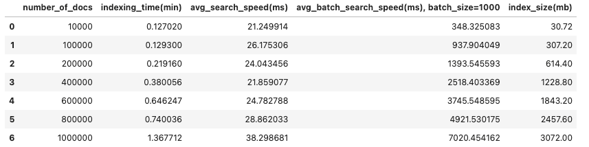
Indexing time in minutes:
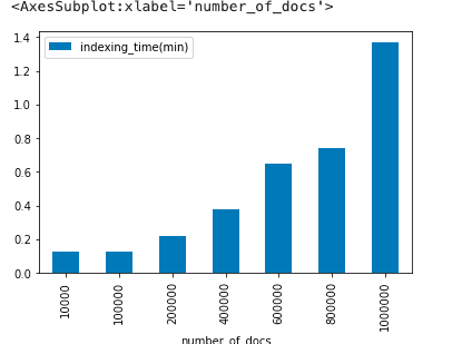
Search speed for single queries:
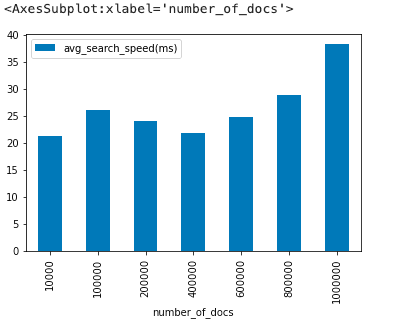
Total search speed for 1,000 queries (batched):
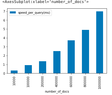
Estimating Per-Query Speed
As mentioned earlier, the results don’t accurately represent the Pinecone engine’s search speed due to network overheard dominating a large part of the final results. However, we can try to estimate the search speed per query without the overheads.
We can view the returned search speeds as:
network_overhead + [num_queries] * [search_speed_per_query]
The network_overhead may change a bit for every call but can be seen as a constant no matter the index size and batch size.
For 1 million documents and assuming the overhead is constant:
Single query:
network_overhead + 1 * search_speed_per_query = 35.68ms
Batched query:
network_overhead + 1000 * search_speed_per_query = 7020.4ms
Solving for search_speed_per_query:
999 * search_speed_per_query = 7020.4 - 35.68 search_speed_per_query = 6.98 ms
Using this logic let’s look at the estimated search speed per query on Pinecone’s engine
Calculating Recall
Recall is an important metric whenever we talk about ANN algorithms since they trade accuracy for speed. Since we do not have ground truth in terms of nearest neighbors for our queries, one way to calculate recall is to compare results between approximate and exact searches.
We calculated recall and approximation-loss as described in our benchmark guide:
Rank-k recall is widespread due to its usage in a standard approximated nearest neighbor search benchmarking tool. It calculates the fraction of approximated (top-k) results with a score (i.e., ‘metric’ score) at least as high as the optimal, exact search, rank-k score. Usually, we robustify the threshold by adding a small ‘epsilon’ number to the rank-k score.
Approximation-loss computes the median top-k ordered score differences between the optimal and approximate-search scores for each test query. In other words, the differences between the optimal and approximate-search top-1 scores, top-2 scores, up to the top-k scores. The final measure is the average of these median values over a set of test queries.
These were the recall and approximation-loss results for 1 million vectors:
Accuracy results over 10 test queries: The average recall @rank-k is 0.991 The median approximation loss is 1.1920928955078125e-07
We saw an average recall of 0.991, which means Pinecone maintains high recall while providing a big boost in search speeds.
Compared Results
Compared to results in the original test, using Pinecone for SBERT embeddings is a way to further improve index sizes, indexing speed, and search speeds.
Pinecone vs. Elasticsearch (vanilla), 1M SBERT embeddings:
- 32x faster indexing
- 5x smaller index size
- 40x faster single-query (non-batched) searches
Pinecone vs. Open Distro for Elasticsearch from AWS, 200k SBERT embeddings:
- 54x faster indexing
- 6x smaller index size
- Over 100ms faster average search speed in batched searches
- 4.4x faster single-query searches
However, note that the HNSW algorithm inside Open Distro can be fine-tuned for higher throughput than seen in the reference article.
Pinecone vs. Elasticsearch with GSI APU plugin, 1M SBERT embeddings:
- 2.4x faster single-query searches
1M SBERT Embeddings
| Indexing Speed (min) | Index Size (GB) | Search Speed (ms) | |
|---|---|---|---|
| Pinecone (batch) | 1.36 | 3 | 6.8 |
| Pinecone (single) | 1.36 | 3 | 38.3 |
| Elasticsearch | 44 | 15 | 1519.7 |
| Elasticsearch + Elastiknn | 51 | 15 | 663.8 |
| Elasticsearch + GSI | 44 | 15 | 92.6 |
200k SBERT Embeddings, Approximate Nearest Neighbors
| Indexing Speed (min) | Index Size (GB) | Search Speed (ms) | |
|---|---|---|---|
| Pinecone (batch) | 0.21 | 0.6 | 1.1 |
| Pinecone (single) | 0.21 | 0.6 | 24.0 |
| Open Distro | 11.25 | 3.6 | 105.7 |
If you would like to benchmark Pinecone for your use case and dataset — for both speed and accuracy — follow our benchmarking guide for vector search services.
Was this article helpful?