How Pinecone Works
Pinecone is a vector database built from the ground up for AI workloads at scale. This page is the definitive technical reference for how Pinecone stores, indexes, and retrieves vectors, covering the serverless object-storage architecture, write and read paths, compaction, metadata filtering, and distributed query execution.For a more detailed deep dive, read the whitepaper.
Architecture Overview
Pinecone is a fully managed, object-storage based vector database. Traditional vector databases require you to provision and manage fixed server clusters. Pinecone takes a different approach: data is stored separately from the machines that process queries. Your vectors live in cloud storage (e.g., Amazon S3), while a flexible pool of processors handles searches. Because these are separate, storage can grow without requiring more processing power, and vice versa. You never need to guess capacity or manage servers.
Fast writes without sacrificing reads
Data is acknowledged in under 100ms and appears in search results within seconds, regardless of index size.
Vectors stored at original quality
Vectors are stored exactly as they are sent, with no data loss. Other systems often compress vectors before storage to save space, permanently reducing accuracy.
Metadata filtering accelerates queries
Selective filters reduce the data scanned, making filtered queries faster than unfiltered ones.
Automatic scaling
Data distributes across immutable files processed in parallel. No parameter tuning, no algorithm selection, no cluster management.
Storage Architecture: The LSM-Based Slab System
Pinecone uses a Log-Structured Merge (LSM) tree approach to organize data. LSM trees are a proven storage pattern designed for write-heavy workloads. The core principle: writes are always sequential. Data is appended to new files rather than modifying existing ones. This makes writes extremely fast and allows reads to happen simultaneously without conflicts.
In Pinecone, the fundamental unit of storage is called a slab.
What is a slab?
A slab is an immutable, self-contained file (or set of files) that holds everything needed to process search queries over the records it contains. It's composed of:
- Raw vectors and metadata stored separately for efficient access
- Vector search indexes with algorithms chosen dynamically based on slab size
- Compressed versions automatically created to reduce size while preserving accuracy
- Sparse vector indexes if records contain sparse vectors
- Metadata bitmap indexes for fast filtered queries
- Manifest file describing contents and structure
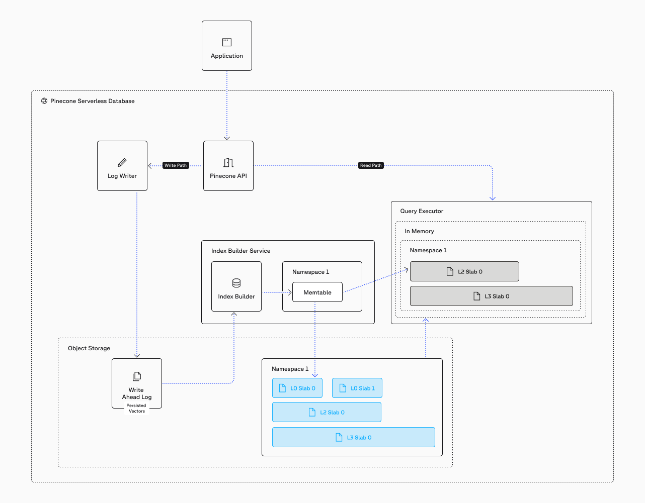
The Write Path: How Data Gets Into Pinecone
Pinecone processes writes in multiple phases, each optimized for a different goal: acknowledgment speed, indexing throughput, and query optimization.
To put throughput in perspective: to saturate the 64MB/s S3 bandwidth limit, you would need to send 32 write operations per second with 300–500 vectors each — over 10,000 vectors per second. Most applications send smaller batches during steady-state streaming writes, and write latency remains consistently low. Pinecone uses brute-force scanning (which is perfectly accurate for up to 10,000 vectors) to serve queries on data that hasn't yet been written to a slab. The index never needs to rebuild or reprocess the entire dataset to incorporate new data.
Write Acknowledgment
When you send a write request (upsert, update, or delete), Pinecone acknowledges it as soon as the operation reaches durable storage. The system writes the operation to a Write-Ahead Log (WAL) on S3 and immediately returns confirmation to your application. Write latency is under 100ms. Each write operation can contain up to 2MB of data in a single batch.
Index Building
After the write reaches S3, the index builder processes it asynchronously per namespace using a consistent hash ring. The index builder pulls up to 10,000 records at a time from the WAL and loads them into a memtable — an in-memory data structure. Records in the memtable are available for querying immediately, even before they flush to disk.
Freshness Guarantees
Updates appear in search results within seconds. The memtable provides immediate access to new data. Background processes handle persistence and optimization without affecting query latency or write throughput. There is no "eventual consistency" window of minutes or hours — seconds is the norm.
Compaction: How Pinecone Optimizes Data in the Background
Each memtable flush creates an L0 slab. L0 slabs are small and fast to create — they contain up to 10,000 records. As L0 slabs accumulate, the compaction process merges them into larger, more optimized structures. Here's how the compaction process works:
How the compaction process works
First write
Your first vector write goes to the WAL. The index builder picks it up, loads it into the memtable, and flushes it to disk as an L0 slab.
L0 slabs accumulate
As more records arrive, they also flush to disk as L0 slabs.
L0 → L1 compaction
When approximately 100 L0 slabs accumulate, compaction gathers the vectors from those slabs and creates a single L1 slab. It writes the L1 slab to disk, notifies the query executors to cache it, and deletes the source L0 slabs.
Partial compaction
If 150 L0 slabs existed when compaction started, 50 L0 slabs and 1 L1 slab remain after compaction. All queries now use those 51 slabs.
L1 → L2 compaction
This repeats with the goal of keeping the total slab count under approximately 100. When more than 100 L1 slabs exist, compaction merges them into L2 slabs.
Steady state
At steady state you might have 10 L0 slabs, 50 L1 slabs, and 3 L2 slabs. Queries use all 63 slabs.
Background operation
While compaction runs, new writes continue creating L0 slabs. Compaction runs continuously in the background.
These are the types of slabs that exist:
L0 Slabs
Up to 10,000 records. Created every memtable flush.
L1 Slabs
~100,000 records. Created when ~100 L0 slabs accumulate.
L2 Slabs
~1,000,000 records. Created when ~100 L1 slabs accumulate.
L3 Slabs
Over 1,000,000 records. Dedicated Read Nodes only.
For on-demand, Pinecone limits the structure to L2 and caps slabs at roughly 10GB. This ensures many reasonably sized files that distribute well across the resource pool. For Dedicated Read Nodes, an additional L3 level is used because each node is dedicated to a single index and can handle larger files. The slab level depends on dataset size, not compaction frequency. As the dataset grows, data flows from many small slabs at higher levels to fewer, larger slabs at lower levels.
Dynamic Algorithm Choices Per-Slab
Because data is automatically partitioned into multiple slabs with different sizes, Pinecone selects the optimal indexing algorithm for each slab independently. You never choose or tune an algorithm — the system selects the best one for each slab based on its characteristics.
The algorithm choice depends on slab size, not slab level. L0 slabs are always Ananas because they're capped at 10,000 records. L1 and L2 slabs use Ananas if small, but switch to IVF when larger. PQFS is being rolled out to replace Ananas at certain large slab sizes. It uses IVF clustering and provides higher recall with lower latency. The roll out is an example of how Pinecone's compaction-based architecture enables transparent algorithmic upgrades — without requiring any changes on your part.
Memtable & small slabs
Brute-force scan. Memtable (up to 10K vectors) lives in RAM, perfectly accurate. Small slabs on disk (up to 100K) are fast enough at this scale to be exact.
Medium slabs (up to 1M)
Ananas — Pinecone's proprietary implementation based on the Fast Johnson-Lindenstrauss Transform (FJLT). Tuned for fast writes and very fast reads.
Large slabs (over 1M)
IVF (Inverted File indexing). Clusters vectors together; each cluster is itself a small Ananas index. Scans only relevant clusters.
The Read Path: Distributed Search and Result Merging
Because every slab is processed independently and in parallel, query latency stays low from millions to billions of vectors.
How a query is processed
The query hits the API gateway, which routes it to the query router.
The query router fans the query out to multiple query executors using a scatter-gather pattern.
Each query executor is responsible for one or more slabs. It processes its assigned slabs locally and in parallel, using the algorithm specified in each slab's manifest.
Each executor returns its local top-k results to the query router.
The query router merges all partial results and returns the global top-k to the client.
System Components: High-Level Data Flow
At a high level, Pinecone's serverless architecture consists of the following components:
Write path
- API Gateway: Receives client requests and routes them to the appropriate path (read or write).
- Index Builder: Processes writes asynchronously. Operates per-namespace using a consistent hash ring to distribute work.
- Write-Ahead Log (WAL): Durable log on object storage (S3). Ensures writes are persisted before acknowledgment.
- Memtable: In-memory structure holding the most recent writes. Queryable immediately. Flushes to L0 slabs.
Read path
- Query Router: Receives queries from the API gateway. Fans them out to query executors and the memtable. Merges partial results into the final top-k.
- Query Executors: Stateless compute nodes that cache slabs on local SSDs. Each executor processes one or more slabs for a given query. The pool of executors scales dynamically.
- Object Storage (S3): The durable backing store for all slabs. Query executors pull slabs from object storage and cache them locally.
Scaling Throughput: Deployment Models
Pinecone offers two deployment models that share the same underlying architecture but optimize for different traffic patterns.
On-Demand
On-Demand indexes use shared infrastructure. Resources scale elastically based on usage, and you pay per read unit consumed. The system handles variable traffic automatically. Ideal for workloads with inconsistent or bursty query patterns — traffic can spike and drop without manual intervention, and you don't pay for idle capacity. Slabs are limited to L2 and capped at roughly 10GB to ensure many reasonably sized files that distribute well across the shared resource pool.
Dedicated Read Nodes (DRN)
DRN indexes run on reserved infrastructure. You provision specific capacity for your index, and pricing is based on the number of shards and replicas you deploy — not query volume. This means you pay the same cost whether you run 100 or 100,000 queries per hour. There is no read unit rate limiting. DRN uses an additional L3 slab level because each node is dedicated to a single index and can handle larger files. Throughput scales independently by adding replicas via API or the Pinecone Console.
Conclusion
Pinecone's serverless, object-storage-based architecture eliminates the tradeoffs that have historically plagued vector search. The LSM-based slab system enables fast writes without sacrificing query performance. Adaptive metadata filtering makes searches faster when filters are selective. Full-fidelity storage preserves accuracy without forcing manual quantization. And background compaction provides continuous, transparent optimization — including algorithmic upgrades — without downtime or re-ingestion.
The result: writes acknowledge in under 100ms, data appears in queries within seconds, and latency stays low from millions to billions of vectors. You don't tune parameters, manage infrastructure, or reduce data fidelity. You build your application, and Pinecone handles the rest.
Download the whitepaper for a deep dive of the architecture.
Frequently Asked Questions
Pinecone uses a serverless architecture built on object storage (such as Amazon S3) with a Log-Structured Merge (LSM) tree-based storage system. Data is stored in immutable files called slabs, and queries are processed by a fleet of stateless query executors that cache slabs on local SSDs. Storage and compute scale independently, eliminating the need to provision or manage fixed infrastructure.
Pinecone stores vectors at full fidelity (full 32-bit precision, any dimension) in immutable files called slabs on object storage. Each slab contains the raw vectors, an ANN index (with the algorithm chosen dynamically based on slab size), bitmap indexes for every metadata field, and a manifest describing the contents. Pinecone applies optimized quantization internally during background compaction — users never need to reduce precision before ingestion.
Pods are Pinecone's legacy architecture. The current Pinecone architecture is serverless, built on object storage with decoupled storage and compute. Pod-based indexes are still supported for existing users, but all new indexes should use the serverless architecture, which offers better scalability, lower operational overhead, and automatic optimization. Pinecone provides migration paths from pods to serverless.
Pinecone acknowledges writes in under 100ms. The system writes operations to a durable Write-Ahead Log (WAL) on S3 and returns confirmation immediately, without waiting for indexing to complete. Data appears in search results within seconds via an in-memory memtable. Each write can contain up to 2MB of data (hundreds of vectors depending on dimensions).
Pinecone indexes every metadata field using roaring bitmaps. At query time, Pinecone dynamically chooses between pre-filtering (scanning only matching records) for selective filters and mid-scan filtering for broad filters. Pinecone never uses traditional post-filtering, which can return fewer than the requested number of results. Selective filters make queries faster, not slower.
No. Pinecone automatically selects the optimal ANN algorithm for each slab based on its size and data characteristics. Small slabs use brute-force scanning, medium slabs use Pinecone's proprietary Ananas algorithm (based on FJLT), and large slabs use IVF indexing. Quantization parameters are also tuned automatically during background compaction. Users do not configure algorithms, cluster topology, or indexing parameters.
On-Demand indexes use shared infrastructure with elastic scaling and per-read-unit pricing — ideal for bursty or variable workloads. Dedicated Read Nodes (DRN) run on reserved infrastructure with flat-fee pricing based on shards and replicas — ideal for sustained high-throughput workloads with no rate limiting. Both share the same underlying storage architecture.
Pinecone partitions each namespace into dozens to hundreds of immutable slabs stored on object storage. At query time, slabs are distributed across a fleet of query executors and processed in parallel using scatter-gather. Because each executor handles only its assigned slabs, the query latency stays low from millions to billions of vectors. The executor pool scales dynamically.
Compaction is a background process that merges smaller slabs into larger, more optimized ones. Small L0 slabs (up to 10K records each) are merged into L1 slabs (~100K records), which are merged into L2 slabs (~1M records). During compaction, Pinecone applies advanced quantization, selects optimal indexing algorithms, and removes tombstoned (deleted/updated) records. Compaction runs continuously without impacting query performance.
No. Pinecone never requires re-indexing. New data is written to new slabs without touching existing ones. Background compaction continuously optimizes the data structures. Even when Pinecone upgrades its indexing algorithms, the improvement is applied transparently during compaction — without downtime, re-ingestion, or user intervention.
Start building knowledgeable AI today
The definitive vector database for AI workloads at scale. Read the full technical whitepaper or start building today.