Pinecone algorithms set new records for BigANN

BigANN is the main competition for large scale vector database algorithms. Pinecone is proud to be a co-organizer of BigANN. We are delighted that strong teams created impressive results that push the boundaries of vector search algorithms. As organizers, we could not participate ourselves. Nevertheless, we invested in creating new algorithms and optimizing known techniques to measure ourselves against the other participants.

We are delighted to report that our methods dominate in all four tracks, with performance that is up to 2x better than the next entry. All tracks required (different) new algorithms and optimizations, some of which are being added to Pinecone’s core database offering. The results and techniques are described below.

Is throughput important?

BigANN is a great competition for fast vector search. But it focuses on throughput (number of queries served per second), which is only one parameter for vector databases, and sometimes not the most important one. This begs the question, why did Pinecone bother to invest in this challenge at all?

Let’s first explain why throughput is not the only important factor for vector databases. Vector databases have a broader range of capabilities and issues they must handle well compared to vector search algorithms competing in BigANN. Vector databases need to provide:

• Consistency and ease of use
• Iron-clad algorithms that work for different workloads
• Support for dynamic insertion and update of data efficiently,
• Low infrastructure costs, including cases with medium or low query throughput, efficient memory use, minimal query SLA variability, operate securely
• Monitoring for operations, billing, disaster recovery, and many other production software considerations

Moreover, the evaluation of recall as a measure of quality, which is used in BigANN, is far too simplistic and sometimes numerically unstable. A proper vector database needs to use several other, more stable, quality metrics for query results.

As a result, the fastests algorithms are not necessarily suitable to operate at the core of a vector database. Nonetheless, our team of research scientists eagerly developed solutions tailored to each track and evaluated their algorithms following the rules of the competition. There were several reasons to do that.

First, we just enjoyed a good challenge. We are scientists and engineers who specialize in high performance computing and algorithms in general and vector search specifically. The opportunity to actually compete with like-minded individuals was too compelling. Second, it was important for us to prove (to ourselves) that if/when we want to optimize solely for throughput, we can do that extremely well. Finally, by competing, we discovered new ideas and optimizations that apply to the core product and will make Pinecone more performant and cost effective.

We plan to release a new benchmarking framework for vector databases soon. The new framework tests vector databases with realistic workloads and requirements.

About BigANN 2023

Let’s dive into the details of the challenge. The BigANN challenge is a competition and a framework for evaluating and advancing the field of Approximate Nearest Neighbor (ANN) search at large scale. The challenge originated in 2019 with a benchmarking effort to standardize the evaluation of ANN algorithms. Following the success of the ANN challenge, in 2021 the BigANN challenge continued the trend to very large datasets (1B vectors), with hybrid in memory-ssd solutions, as well as custom hardware for ANN.

This year, the focus was on moderately-sized datasets (10M vectors), but with additional features related to real-world usability of ANN: metadata filters, sparse vectors, streaming setting, and out-of-distribution (OOD), which are the four tracks of the challenge.

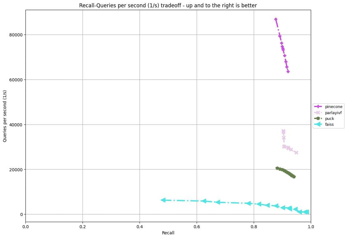
The Filter track uses a dataset of 10M vectors (a 10M slice of the YFCC 100M dataset), where every image in the dataset was embedded using a variant of the CLIP embedding. Every image (vector) is associated with a set of tags: words extracted from the description, the camera model, the year the picture was taken and the country. The tags are from a vocabulary of 200386 possible tags. The 100,000 queries consist of one image embedding and one or two tags that must appear in the database elements to be considered. Submissions are evaluated based on highest throughput where the recall@10 is at least 90%.

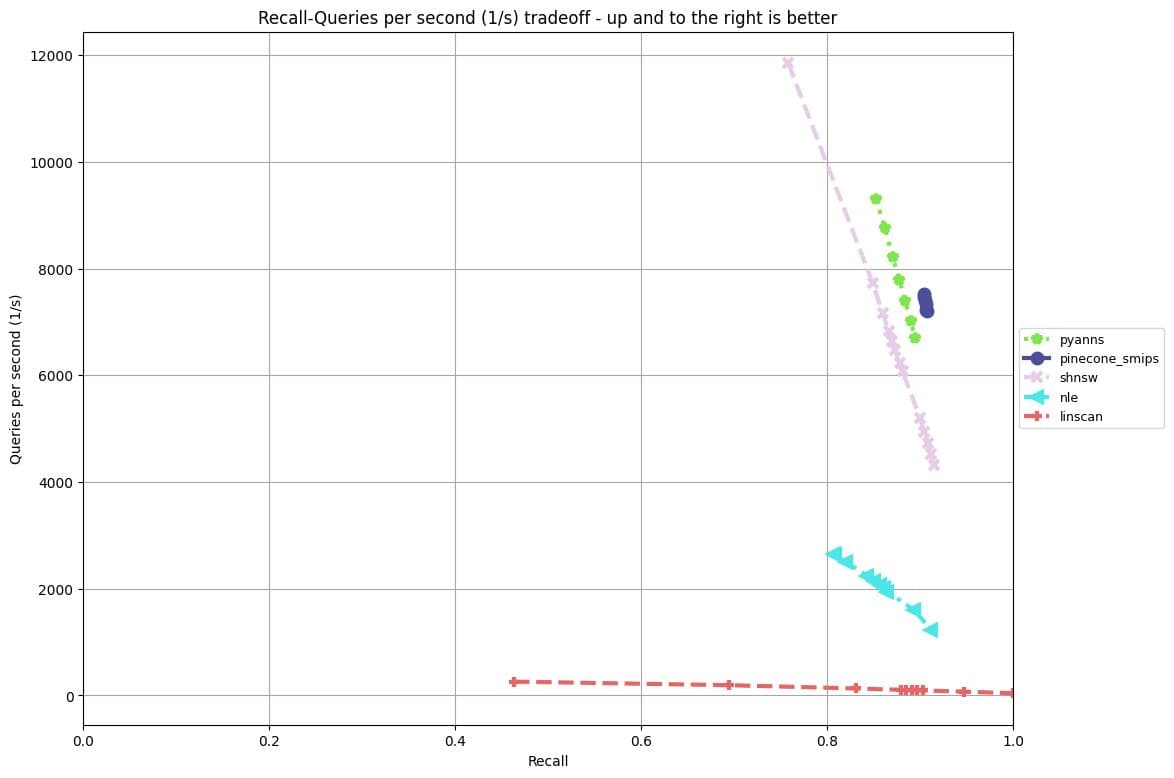
In the Sparse track, vectors are high-dimensional (roughly 30,000 dimensions) but have very few non-zero coordinates (about 120 per data point, 40 per query point). The vector collection is, in fact, an embedding of the MS MARCO Passage corpus with the SPLADE model; a powerful neural model that learns robust, sparse representations of text data. As in the filter track, submissions are evaluated based on highest throughput past 90% recall.

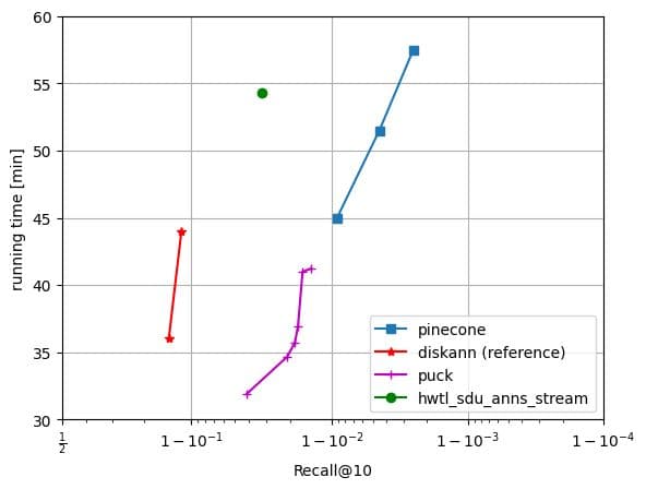
The Streaming track begins with an empty set. Over the course of at most one hour and utilizing a maximum of 8 GB of main memory, solutions are expected to execute the "runbook" provided, an interleaved sequence of insertions, deletions, and top-10 search requests, with data points coming from a 30 million item slice of the MS Turing dataset. The runbook assesses the adaptability of an indexing algorithm to draft data. Submissions are evaluated based on average recall across all search requests.

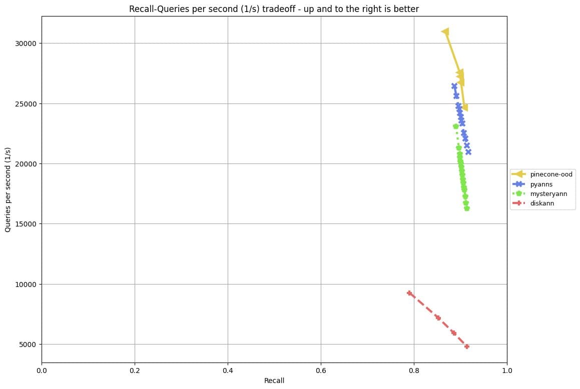
Finally, the Out-Of-Distribution (OOD) track involves traditional high-dimensional ANN search but with queries drawn from a different distribution than the indexed vectors – capturing the cross-modal search setting. The vector collection is a 10 million sized sample of the Yandex Text-to-Image dataset, corresponding to 200-dimensional image embeddings of images from Yandex’s visual search engine embedded with the Se-ResNext-101 model. The queries are embeddings of textual queries into the same representation space, embedded using a variant of the DSSM model. Like the Sparse and Filter Tracks, submissions are ranked based on the throughput of their solutions that achieve at least 90% recall.

Our Results

All the results below follow the BigANN competition evaluation framework and guideline, ensuring a fair comparison (see more details below). In tracks where there is a hidden query set (Filter and Sparse), we optimized any hyperparameters on the public query set, and only then evaluated on the hidden query set.

Filter track

Comparison of our Filter track solution against the official baseline (faiss) and top contenders on the hidden query set. At 90% recall, our throughput is roughly 74,000 qps, which is approximately 2x the next best submission, parlayivf, at 37,000 qps.

Sparse track

Comparison of our Sparse track solution against the official baseline (linscan) and top three contenders on the hidden query set. At 90% recall, our throughput is roughly 7,500 qps versus pyanns’s approximately 6,400 qps. We highlight that the NLE solution performs half as fast on the test set as it does on the dev set, while other methods are more consistent and less sensitive to the query set.

OOD Track

Comparison of our OOD track solution against the official baseline (diskann) and top contenders (on the public query set since on this track there is no hidden query set). At 90% recall, our throughput is roughly 27,200QPS, vs the top contender, pyanns, at approximately 23,000 qps.

Streaming track

Comparison of our Streaming track solution against the official baseline and top contender. Our algorithm achieves a recall of 0.9975 under the 60 minutes limit, compared to 0.986 of the best contender. Here too, there is no private query set. These runs are on the official runbook named final_runbook.yaml.

Algorithm details

Filter track:

Our algorithm is based on the classical IVF architecture, where the data is first divided into geometrical clusters, combined with a metadata inverted index: for every metadata tag, we store a list of vectors with that tag.

Given a query, we first evaluate its level of selectivity (i.e., the count of vectors that pass the filter), and scan a varying number of clusters for that query. We efficiently scan only the relevant vectors based on the inverted index, so the number of operations is O(query selectivity) rather than O(# of vectors in the selected clusters). The intuition is that for wide queries, the closest vectors are in neighboring clusters, and for more selective queries there is a need to scan more clusters. Additionally, we make sure that a minimal number of relevant vectors have been scanned, to account for queries whose selectivity is less localized.

To accelerate the search, we pre-compute some of the intersections of the inverted lists (based on their size), and use AVX for efficient computation of distances. To optimize the hyperparameters on the public query set, we formalized the problem as a constrained convex optimization problem, assigning the optimal recall value for each selectivity bucket. For the most selective queries, it turns out that it is beneficial to simply scan all relevant vectors (and ignore the geometrical clustering).

Sparse track

Our algorithm for the Sparse track is based on our very own research [1, 2]. In particular, we cluster sparse vectors, build an inverted index that is organized using our novel structure, and query the index by first solving the top cluster retrieval problem, then finding the top-k vectors within those clusters using an anytime retrieval algorithm over the inverted index.

We also augment the index above with two additional lightweight components. First, we use a k-MIP graph (where every vector is connected to k other vectors that maximize inner product with it) to “expand” the set of retrieved top-k vectors from the last step. Second, we re-rank the expanded set using a compressed forward index. In effect, our final solution is a hybrid of IVF- and graph-based methods, where the IVF stage provides a set of entry nodes into the graph.

OOD track

Our solution for the OOD track is similar in flavor to our approach in the Sparse track but different in some key ways. We build three main components – an inverted-file (IVF) index on the vector collection using a clustering algorithm tailored for inner-product search, a k-MIP graph constructed using the co-occurence of vectors as nearest neighbors for a set of training queries, and, quantization tailored for SIMD-based acceleration for fast scoring and retrieval.

We perform retrieval in three stages. First, we retrieve a small number of candidates from top clusters by scoring quantized vectors. Next, we use the k-MIP graph to “expand” the set of retrieved candidates by adding their neighbors in the graph to the candidate set. Finally, we score all the candidates by computing their distance to the query using a fine-grained quantized representation of the vectors. In addition, in order to accelerate the search, we process the queries in a batch to take advantage of cache locality.

Streaming track

Our solution employs a two-stage retrieval strategy. In the initial phase, we use a variant of the DiskANN index for candidate generation to generate a set of k’ >> k results through an approximate scoring mechanism over uint8-quantized vectors, with accelerated SIMD-based distance calculation. The second-stage reranks the candidates using full-precision scoring to enhance the overall accuracy of retrieval. It is worth noting that the raw vectors used in the second stage are stored on SSD. As such, it is important to optimize the number of disk reads invoked by the reranking stage.

Evaluation Metrics and Methodology

Here we add additional details about our setup and how we ensure a fair comparison between the official submissions and our own solutions.

In the Filter, Sparse and OOD tracks, the evaluation metric is maximum QPS at recall@10 of at least 0.9. The Filter and Sparse track have a hidden query set, which was not used during the algorithm development or hyperparameter tuning. For the Streaming track, the metric is the maximum recall@10, where the algorithm must execute, within an hour, a runbook containing insertion, deletion and queries, simulating a production load of a vector database.

All our experiments were conducted on the standard BigANN evaluation VM (Azure Standard D8lds v5 with 8 vcpus and 16 GiB memory). All the results shown in the plots (including competing algorithms) were reproduced on the same machine.

The code for our solutions is not planned to be released at this time. Pinecone’s database is closed source and provided as a managed service. Nevertheless, we have released the binaries of the submitted algorithm so that everyone can verify our results, these can be accessed from the bigann repository.

Are these new algorithms powering pinecone’s vector index?

These algorithms represent the state-of-the-art in each of the tracks, which are focused on in-memory algorithms. Pinecone’s vector database works in a managed cloud environment. It has many constraints which the BigANN competition does not share. As a result, these solutions are actually not the most efficient in production workloads. Nevertheless, there are several components that are a part of Pinecone’s database and some that were developed as part of the challenge that will be integrated into the product.

Conclusions

The recent BigANN challenge emphasized new features vital for advancing vector database research and bridging academic and industrial efforts. However, designing vector databases for real-world applications involves further aspects. Key considerations include cost efficiency (memory and disk space usage) and data freshness (speed of update reflection in queries). A robust production-grade database must integrate these elements (such as filter queries, sparse vectors, and data freshness). Future challenges are anticipated to encompass these additional factors. Nevertheless, we enjoyed working on this challenge, and are incorporating some of the new algorithms and components in the pinecone vector index.