# How Spotify Uses Semantic Search for Podcasts
> Want to add audio search to your applications just like Spotify? You’ll need a vector database like Pinecone. Try it now for free.
**Want to add audio search to your applications just like Spotify? You’ll need a vector database like** **[Pinecone](https://www.pinecone.io/).** [Try it now for free.](https://app.pinecone.io/)
The market for podcasts has grown tremendously in recent years, with the number of global listeners having increased by 20% annually in recent years [1].
Driving the charge in podcast adoption is Spotify. In a few short years, they have become the undisputed leaders in podcasting. Despite only entering the game in 2018, by late 2021, Spotify had already usurped Apple, the long-reigning leader in podcasts, with more than 28M monthly podcast listeners [2]
To back their podcast investments, Spotify has worked on making the podcast experience as seamless and accessible as possible. From their all-in-one podcast creation app (Anchor) to podcast APIs and their latest _natural language enabled_ podcast search.
Spotify’s natural language search for podcasts is a fascinating use case. In the past, users had to rely on keyword/term matching to find the podcast episodes they wanted. Now, they can search in natural language, in much the same way we might ask a real person where to find something.
This technology relies on what we like to call _semantic search_. It enables a more intuitive search experience because we tend to have an _idea_ of what we’re looking for, but rarely do we know precisely which terms appear in what we want.
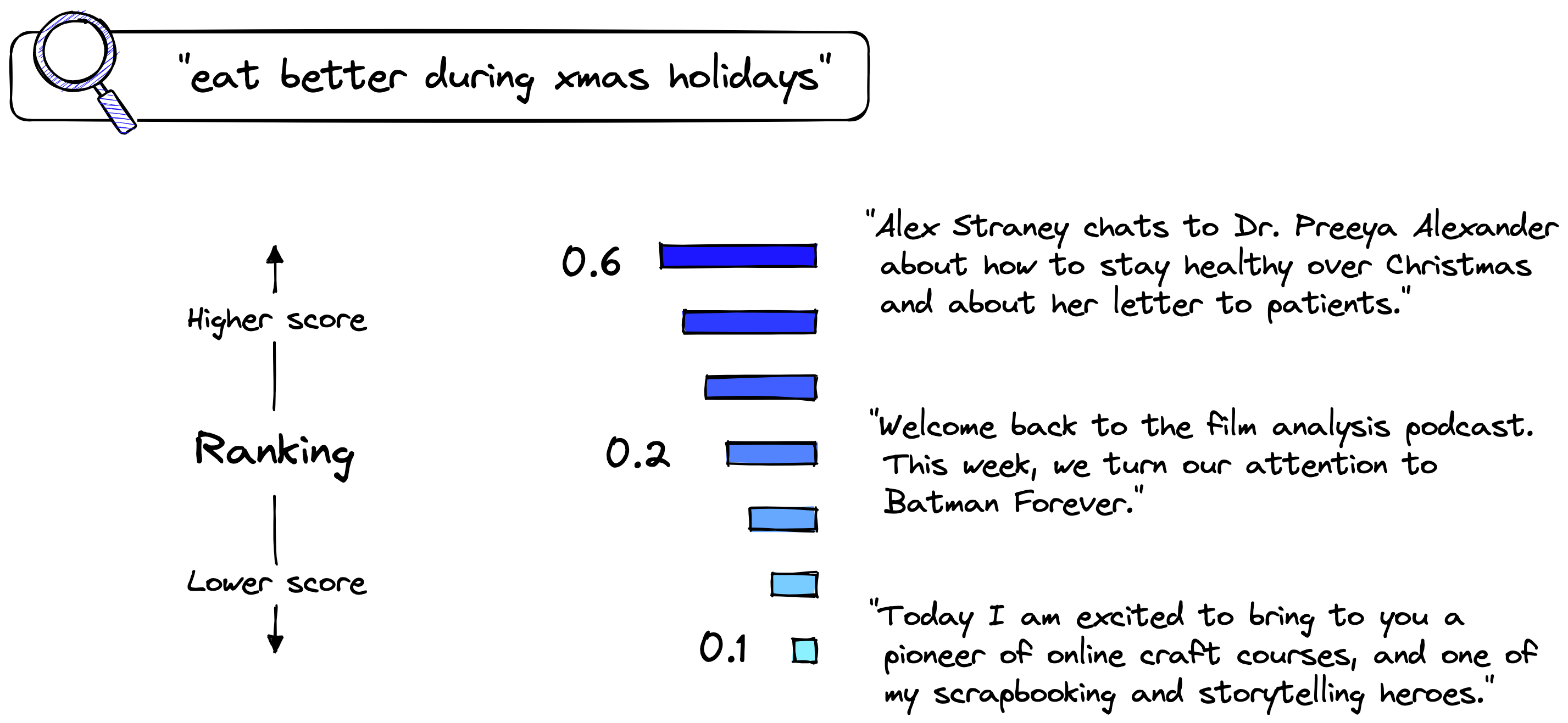
Imagine we wanted to find a podcast talking about healthy eating over the holidays. How would we search for that? It might look something like:

There is a podcast episode talking about precisely this. Its description is:
```
"Alex Straney chats to Dr. Preeya Alexander about how to stay healthy over Christmas and about her letter to patients."
```
We have zero overlaps between the query and episode description using term matching, so this result would not be returned using keyword search. To make matters worse, there are undoubtedly thousands of episode descriptions on Spotify containing the words _“eat”_, _“better”_, and _“holidays”_. These episodes likely have nothing to do with our intended search query, but we could return them.
Suppose we were to swap that for a semantic search query. We could see much better results because semantic search looks at the meaning of the words and sentences, _not_ specific terms.
Despite sharing no words, our query and episode description would be identified as having very similar meanings. They both describe _being or eating healthier over the winter holidays_.
Enabling meaningful search is not easy, but the impact can be huge if done well. As Spotify has proven, it can lead to a much greater user experience. Let’s dive into how Spotify built its natural language podcast search.
[Video](https://www.youtube.com/watch?v=ok0SDdXdat8)
## Semantic Search
The technology powering Spotify’s new podcast search is more widely known as semantic search. Semantic search relies on two pillars, [Natural](https://www.pinecone.io/learn/series/nlp/) [Language](https://www.pinecone.io/learn/series/nlp/) [Processing (NLP)](https://www.pinecone.io/learn/series/nlp/) and [vector search](https://www.pinecone.io/learn/vector-search-basics/).
These technologies act as two steps in the search process. Given a natural language query, a particular NLP model can encode it into a [vector embedding](https://www.pinecone.io/learn/vector-embeddings/), also known as a [dense vector](https://www.pinecone.io/learn/series/nlp/dense-vector-embeddings-nlp/). These dense vectors can numerically represent the meaning of the query.
```json
{
"_key": "1cdad8e5eb2e",
"_type": "plotlyPlot",
"asset": {
"_ref": "file-22c86373ed140a7d4bfe4ebd40346f3bb00dfc38-json",
"_type": "reference"
}
}
```
These vectors have been encoded by one of these special NLP models, called [sentence transformers](https://www.pinecone.io/learn/series/nlp/sentence-embeddings/). We can see that queries with similar meanings cluster together, whereas unrelated queries do not.
Once we have these vectors, we need a way of comparing them. That is where the _vector search_ component is used. Given our new query vector, we perform a vector search and compare it to previously encoded vectors and retrieve those that are nearest or the most similar.
NLP and vector search have been around for some time, but recent advancements have acted as catalysts in the performance increase and subsequent adoption of semantic search. In NLP, we have seen the introduction of high-performance [transformer models](https://www.pinecone.io/learn/transformers/). In vector search, the rise of **A**pproximate **N**earest **N**eighbor (ANN) algorithms.
Transformers and ANN search have powered the growth of semantic search, but _why_ is not so clear. So, let’s demystify how they work and why they’ve proven so helpful.
### Transformers
Transformer models have become the standard in NLP. These models typically have two components: the core, which focuses on _“understanding”_ the meaning of a language and/or domain, and a head, which adapts the model for a particular use case.
There is just one problem, the core of these models requires vast amounts of data and computing power to pretrain.
---
_Pretraining refers to the training step applied to the core transformer component. It is followed by a fine-tuning step where the head and/or the core are trained further for a specific use case._
---
One of the most popular transformer models is BERT, and BERT costs a reported 2.5K - 50K (USD) to train; this shifts to 80K - 1.6M (USD) for the larger BERT model [4].
These costs are prohibitive for most organizations. Fortunately, that doesn’t stop us from using them. Despite these models being expensive to pretrain, they are an order of magnitude cheaper to _fine-tune_.
The way that we would typically use these models is:
1. The core of the transformer model is pretrained at great cost by the likes of Google, Microsoft, etc.
2. This core is made publicly available.
3. Other organizations take the core, add a task-specific _“head”_, and fine-tune the extended model to their domain-specific task. Fine-tuning is less computationally expensive and therefore cheaper.
4. The model is now ready to be applied to the organization’s domain-specific tasks.
In the case of building a podcast search model, we could take a pretrained model like `bert-base-uncased`. This model already “understands” general purpose English language.
Given a training dataset of _user query_ to _podcast episode_ pairs, we could add a _“mean pooling”_ head onto our pretrained BERT model. With both the core and head, we fine-tune it for a few hours on our pairs data to create a _sentence_ transformer trained to identify similar query-episode pairs.
We must choose a suitable pretrained model for our use case. In our example, if our target query-episode pairs were English language only, it would make no sense to take a French pretrained model. It has no base understanding of the English language and could not learn to understand the English query-episode pairs.
Another term we have mentioned is _“sentence transformer”_. This term refers to a transformer model that has been fitted with a pooling layer that enables it to output single vector representations of sentences (or longer chunks of text).
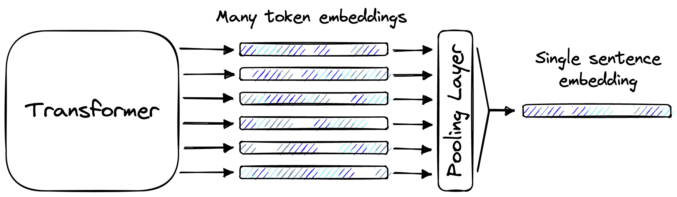
There are different types of pooling layers, but they all consume the same input and produce the same output. They take many token-level embeddings and merge them in some way to build a single embedding that represents _all_ of those token-level embeddings. That single output is called a _sentence embedding_.
The sentence embedding is a _dense vector_, a numerical representation of the meaning behind some text. These dense vectors enable the _vector search_ component of semantic search.
### ANN Search
**A**pproximate **N**earest **N**eighbors (ANN) search allows us to quickly compare millions or even billions of vectors. It is called _approximate_ because it does not guarantee that we will find the true nearest neighbors (most similar embeddings).
The only way we can guarantee that is by exhaustively comparing every single vector. At scale, that’s slow.
Rather than comparing _every_ vector, we approximate with ANN search. If done well, this approximation can be incredibly accurate and super fast. But there is often a trade-off. Some algorithms offer speedier search but poorer accuracy, whereas others may be more accurate but increase search times.
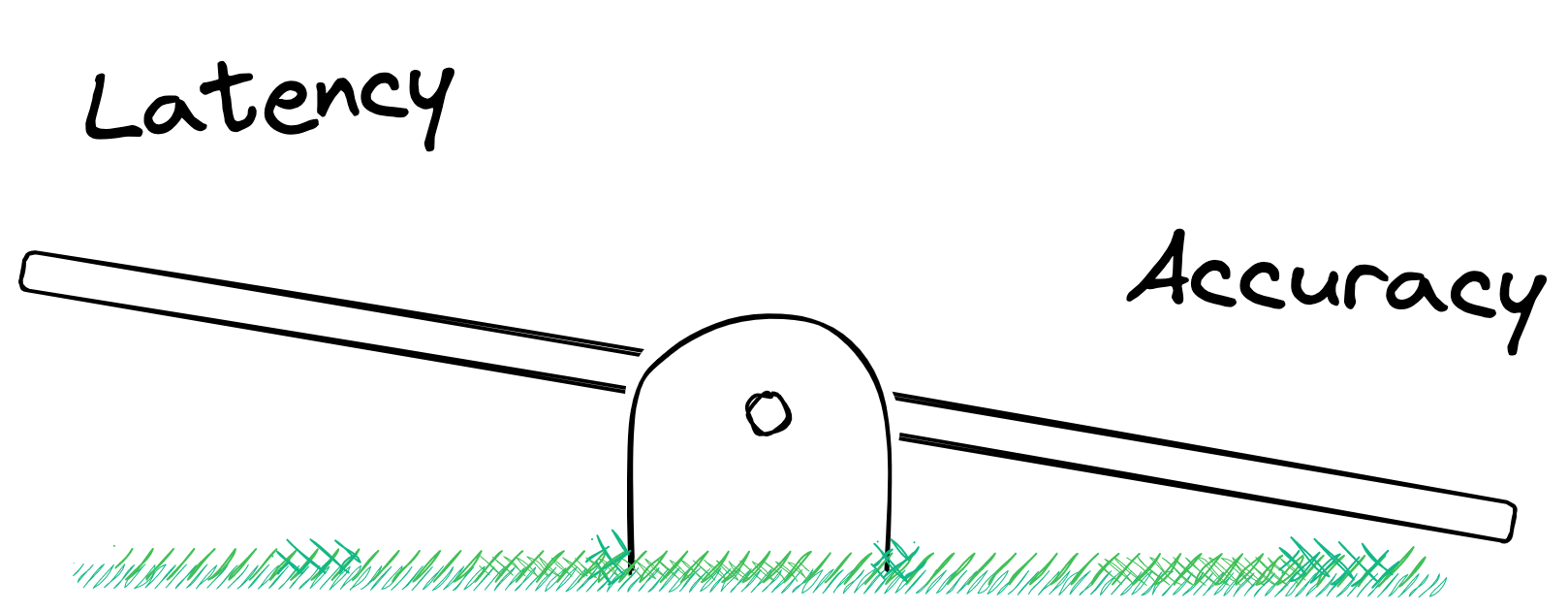
In either case, an approximate solution is required to maintain reasonable query times at scale.
## How Spotify Did It
To build this type of semantic search tool, Spotify needed a language model capable of encoding similar _(query, episode)_ pairs into a similar vector space. There are existing sentence transformer [models like SBERT](https://www.pinecone.io/learn/series/nlp/train-sentence-transformers-softmax/), but Spotify found two issues with using this model:
- They needed a model capable of supporting multilingual queries; SBERT was trained on English text only.
- SBERT’s cross-topic performance _without_ further fine-tuning is poor [5].
With that in mind, they decided to use a different, multilingual model called the **U**niversal **S**entence **E**ncoder (USE). But this still needed fine-tuning.
To fine-tune their USE model to encode _(query, episode)_ pairs in a meaningful way, Spotify needed _(query, episode)_ data. They had _four_ sources of this:
1. Using their past search logs, they identified _(query, episode)_ pairs from successful searches.
2. They identified unsuccessful searches that were followed by a successful search. The idea is that the unsuccessful query is likely to be a more _natural_ query, which was then used as a _(query_prior_to_successful_reformulation, episode)_ pair.
3. Generating synthetic queries using a query generation model produces _(synthetic_query, episode)_ pairs.
4. A small set of curated queries, manually written for episodes.
Sources (1 - 3) fine-tune the USE model, with some samples left for evaluation. Source (4) was used for evaluation only.
Unfortunately, we don’t have access to Spotify’s past search logs, so there’s little we can do in replicating sources (1 - 2). However, we can replicate the approach of the building source (3) using query generation models. And, of course, we can manually write queries as per source (4).
### Data Preprocessing
Before generating any queries, we need episode data. Spotify describes _episodes_ as a concatenation of textual metadata fields, including episode title and description, with the podcast show’s title and description.
We can find a [podcast episodes dataset](https://www.kaggle.com/datasets/listennotes/all-podcast-episodes-published-in-december-2017) on Kaggle that contains records for 881k podcast episodes i. Including episode titles and descriptions, with podcast show titles and descriptions.
We use the Kaggle API to download this data, installed in Python with `pip install kaggle`. An account and API key are needed (find the API key in your _Account Settings_). The _kaggle.json_ API key should be stored in the location displayed when attempting to `import kaggle`. If no location or error appears, the API key has already been added.
We then authenticate access to Kaggle.
```python
from kaggle.api.kaggle_api_extended import KaggleApi
api = KaggleApi()
api.authenticate()
```
Once authenticated, we can download the dataset using the `dataset_download_file` function, specifying the dataset location (found from its URL), files to download, and where to save them.
```python
api.dataset_download_file(
'listennotes/all-podcast-episodes-published-in-december-2017',
file_name='podcasts.csv',
path='./'
)
api.dataset_download_file(
'listennotes/all-podcast-episodes-published-in-december-2017',
file_name='episodes.csv',
path='./'
)
```
Both _podcasts.csv_ and _episodes.csv_ will be downloaded as zip files, which we can extract using the `zipfile` library.
```python
with zipfile.ZipFile('podcasts.csv.zip', 'r') as zipref:
zipref.extractall('./')
with zipfile.ZipFile('episodes.csv.zip', 'r') as zipref:
zipref.extractall('./')
```
We have two CSV files, _podcasts.csv_ details the podcast shows themselves, including titles, descriptions, and hosts. The _episodes.csv_ data includes data from specific podcast episodes, including episode title, description, and publication date.
To replicate Spotify’s approach of concatenating podcast shows and episode-specific details, we must merge the two datasets. We do this with an inner join on the podcast ID columns.
```python
episodes = episodes.merge(
podcasts,
left_on='podcast_uuid',
right_on='uuid',
suffixes=('_ep', '_pod')
)
```
Before concatenating the features we want, let’s clean up the data. We strip excess whitespace and remove rows where _any_ of our relevant features contain null values.
```json
{
"_key": "1bd60120b68d",
"_type": "colabBlock",
"jsonContent": "{\n \"cells\": [\n {\n \"cell_type\": \"code\",\n \"execution_count\": 4,\n \"metadata\": {},\n \"outputs\": [],\n \"source\": [\n \"features = ['title_ep', 'description_ep', 'title_pod', 'description_pod']\\n\",\n \"# strip whitespace\\n\",\n \"episodes[features] = episodes[features].apply(lambda x: x.str.strip())\"\n ]\n },\n {\n \"cell_type\": \"code\",\n \"execution_count\": 5,\n \"metadata\": {},\n \"outputs\": [\n {\n \"name\": \"stdout\",\n \"output_type\": \"stream\",\n \"text\": [\n \"Before: 873820\\n\",\n \"After: 778182\\n\"\n ]\n }\n ],\n \"source\": [\n \"print(f\\\"Before: {len(episodes)}\\\")\\n\",\n \"episodes = episodes[\\n\",\n \" ~episodes[features].isnull().any(axis=1)\\n\",\n \"]\\n\",\n \"print(f\\\"After: {len(episodes)}\\\")\"\n ]\n }\n ],\n \"metadata\": {\n \"environment\": {\n \"kernel\": \"python3\",\n \"name\": \"common-cu110.m91\",\n \"type\": \"gcloud\",\n \"uri\": \"gcr.io/deeplearning-platform-release/base-cu110:m91\"\n },\n \"interpreter\": {\n \"hash\": \"5188bc372fa413aa2565ae5d28228f50ad7b2c4ebb4a82c5900fd598adbb6408\"\n },\n \"kernelspec\": {\n \"display_name\": \"Python 3\",\n \"language\": \"python\",\n \"name\": \"python3\"\n },\n \"language_info\": {\n \"codemirror_mode\": {\n \"name\": \"ipython\",\n \"version\": 3\n },\n \"file_extension\": \".py\",\n \"mimetype\": \"text/x-python\",\n \"name\": \"python\",\n \"nbconvert_exporter\": \"python\",\n \"pygments_lexer\": \"ipython3\",\n \"version\": \"3.8.8\"\n }\n },\n \"nbformat\": 4,\n \"nbformat_minor\": 4\n}"
}
```
We’re ready to concatenate, giving us our _episodes_ feature.
```json
{
"_key": "d612ba1a4a32",
"_type": "colabBlock",
"jsonContent": "{\n \"cells\": [\n {\n \"cell_type\": \"code\",\n \"execution_count\": 6,\n \"metadata\": {},\n \"outputs\": [],\n \"source\": [\n \"episodes = episodes['title_ep'] + '. ' + episodes['description_ep'] + '. ' \\\\\\n\",\n \" + episodes['title_pod'] + '. ' + episodes['description_pod']\\n\",\n \"episodes = episodes.to_list()\"\n ]\n },\n {\n \"cell_type\": \"code\",\n \"execution_count\": 7,\n \"metadata\": {},\n \"outputs\": [\n {\n \"data\": {\n \"text/plain\": [\n \"['Fancy New Band: Running Stitch. Running Stitch join Hannah to play sme new tracks ahead of their EP release next year. Cheers NZ On Air Music!
. 95bFM. Audio on demand from selected shows',\\n\",\n \" \\\"Political Commentary w/ David Slack: December 21, 2017. It's the end of the year, and let's face it... 2017 hasn't been a great one for empathy. From\\\\xa0the public treatment of our politicians\\\\xa0to the treament of our least fortunate citizens, David Slack reckons it's about time we all took pause. It is Christmas, after all.
. 95bFM. Audio on demand from selected shows\\\",\\n\",\n \" 'From the Crate w/ Troy Ferguson: December 21, 2017. LP exploration with the ever-knowledgeable Troy, featuring the following new cakes and/or tasty re-releases:
\\\\n\\\\n\\\\n\\\\t- Ken Boothe - You Keep Me Hangin\\\\' On
\\\\n\\\\t- The New Sounds -\\\\xa0The Big Score
\\\\n\\\\t- Jitwam -\\\\xa0Keepyourbusinesstoyourself
\\\\n
\\\\n\\\\nAll available from and thanks to\\\\xa0Southbound Records.
. 95bFM. Audio on demand from selected shows']\"\n ]\n },\n \"execution_count\": 7,\n \"metadata\": {},\n \"output_type\": \"execute_result\"\n }\n ],\n \"source\": [\n \"episodes[50:53]\"\n ]\n },\n {\n \"cell_type\": \"markdown\",\n \"metadata\": {},\n \"source\": [\n \"Let's shuffle our data too.\"\n ]\n },\n {\n \"cell_type\": \"code\",\n \"execution_count\": 8,\n \"metadata\": {},\n \"outputs\": [],\n \"source\": [\n \"from random import shuffle\\n\",\n \"\\n\",\n \"shuffle(episodes)\"\n ]\n }\n ],\n \"metadata\": {\n \"environment\": {\n \"kernel\": \"python3\",\n \"name\": \"common-cu110.m91\",\n \"type\": \"gcloud\",\n \"uri\": \"gcr.io/deeplearning-platform-release/base-cu110:m91\"\n },\n \"interpreter\": {\n \"hash\": \"5188bc372fa413aa2565ae5d28228f50ad7b2c4ebb4a82c5900fd598adbb6408\"\n },\n \"kernelspec\": {\n \"display_name\": \"Python 3\",\n \"language\": \"python\",\n \"name\": \"python3\"\n },\n \"language_info\": {\n \"codemirror_mode\": {\n \"name\": \"ipython\",\n \"version\": 3\n },\n \"file_extension\": \".py\",\n \"mimetype\": \"text/x-python\",\n \"name\": \"python\",\n \"nbconvert_exporter\": \"python\",\n \"pygments_lexer\": \"ipython3\",\n \"version\": \"3.8.8\"\n }\n },\n \"nbformat\": 4,\n \"nbformat_minor\": 4\n}"
}
```
### Query Generation
We now have episodes but no queries, and we need _(query, episode)_ pairs to fine-tune a model. Spotify generated synthetic queries from episode text, which we can do.
To do this, they fine-tuned a query generation BART model using the MS MARCO dataset. We don’t need to fine-tune a BART model as plenty of readily available models have been fine-tuned on the exact same dataset. Therefore, we will initialize one of these models using the HuggingFace _transformers_ library.
```python
from transformers import T5Tokenizer, T5ForConditionalGeneration
# after testing many BART and T5 query generation models, this seemed best
model_name = 'doc2query/all-t5-base-v1'
tokenizer = T5Tokenizer.from_pretrained(model_name)
model = T5ForConditionalGeneration.from_pretrained(model_name).cuda()
```
We tested several T5 _and_ BART models for query generation on our episodes data; the [results are here](https://github.com/pinecone-io/examples/blob/master/learn/search/semantic-search/spotify-podcast-search/query-gen.md). The `doc2query/all-t5-base-v1` model was chosen as it produced more reasonable queries and has some multilingual support.
It’s time for us to generate queries. We will generate three queries per episode, in-line with the approach taken by the [GenQ](https://www.pinecone.io/learn/series/nlp/genq/) and [GPL](https://www.pinecone.io/learn/series/nlp/gpl/) techniques.
```json
{
"_key": "515132ee7db7",
"_type": "colabBlock",
"jsonContent": "{\n \"cells\": [\n {\n \"cell_type\": \"code\",\n \"execution_count\": 10,\n \"metadata\": {},\n \"outputs\": [],\n \"source\": [\n \"# (OPTIONAL) it will take a long time to produce queries for the entire dataset, let's drop some episodes\\n\",\n \"episodes = episodes[:100_000]\"\n ]\n },\n {\n \"cell_type\": \"code\",\n \"execution_count\": 11,\n \"metadata\": {},\n \"outputs\": [\n {\n \"data\": {\n \"application/vnd.jupyter.widget-view+json\": {\n \"model_id\": \"2ed4811ef70d478280550edcb16d1859\",\n \"version_major\": 2,\n \"version_minor\": 0\n },\n \"text/plain\": [\n \"100%|██████████| 100000/100000 [08:44:31<00:00]\"\n ]\n },\n \"metadata\": {},\n \"output_type\": \"display_data\"\n }\n ],\n \"source\": [\n \"from tqdm.auto import tqdm\\n\",\n \"\\n\",\n \"batch_size = 128 # larger batch size == faster processing\\n\",\n \"num_queries = 3 # number of queries to generate for each episode\\n\",\n \"pairs = []\\n\",\n \"ep_batch = []\\n\",\n \"\\n\",\n \"for ep in tqdm(episodes):\\n\",\n \" # remove tab + newline characters if present\\n\",\n \" ep_batch.append(ep.replace('\\\\t', ' ').replace('\\\\n', ' '))\\n\",\n \" \\n\",\n \" # we encode in batches\\n\",\n \" if len(ep_batch) == batch_size:\\n\",\n \" # tokenize the passage\\n\",\n \" inputs = tokenizer(\\n\",\n \" ep_batch,\\n\",\n \" truncation=True,\\n\",\n \" padding=True,\\n\",\n \" max_length=256,\\n\",\n \" return_tensors='pt'\\n\",\n \" )\\n\",\n \"\\n\",\n \" # generate three queries per episode\\n\",\n \" outputs = model.generate(\\n\",\n \" input_ids=inputs['input_ids'].cuda(),\\n\",\n \" attention_mask=inputs['attention_mask'].cuda(),\\n\",\n \" max_length=64,\\n\",\n \" do_sample=True,\\n\",\n \" top_p=0.95,\\n\",\n \" num_return_sequences=num_queries\\n\",\n \" )\\n\",\n \"\\n\",\n \" # decode query to human readable text\\n\",\n \" decoded_output = tokenizer.batch_decode(\\n\",\n \" outputs,\\n\",\n \" skip_special_tokens=True\\n\",\n \" )\\n\",\n \"\\n\",\n \" # loop through to pair query and episodes\\n\",\n \" for i, query in enumerate(decoded_output):\\n\",\n \" query = query.replace('\\\\t', ' ').replace('\\\\n', ' ') # remove newline + tabs\\n\",\n \" ep_idx = int(i/num_queries) # get index of episode to match query\\n\",\n \" pairs.append([query, ep_batch[ep_idx]])\\n\",\n \" \\n\",\n \" ep_batch = []\"\n ]\n }\n ],\n \"metadata\": {\n \"environment\": {\n \"kernel\": \"python3\",\n \"name\": \"common-cu110.m91\",\n \"type\": \"gcloud\",\n \"uri\": \"gcr.io/deeplearning-platform-release/base-cu110:m91\"\n },\n \"interpreter\": {\n \"hash\": \"5188bc372fa413aa2565ae5d28228f50ad7b2c4ebb4a82c5900fd598adbb6408\"\n },\n \"kernelspec\": {\n \"display_name\": \"Python 3\",\n \"language\": \"python\",\n \"name\": \"python3\"\n },\n \"language_info\": {\n \"codemirror_mode\": {\n \"name\": \"ipython\",\n \"version\": 3\n },\n \"file_extension\": \".py\",\n \"mimetype\": \"text/x-python\",\n \"name\": \"python\",\n \"nbconvert_exporter\": \"python\",\n \"pygments_lexer\": \"ipython3\",\n \"version\": \"3.8.8\"\n }\n },\n \"nbformat\": 4,\n \"nbformat_minor\": 4\n}"
}
```
Query generation can take some time, and we recommend limiting the number of episodes (we used 100k in this example). Looking at the generated queries, we can see some good and some bad. This randomness is the nature of query generation and should be expected.
We now have _(synthetic_query, episode)_ pairs that can be used in fine-tuning a sentence transformer model.
### Models and Fine-tuning
As mentioned, Spotify considered using pretrained models like BERT and SBERT but found the performance unsuitable for their use case. In the end, they opted for a pretrained **U**niversal **S**entence **E**ncoder (USE) model from TFHub.
We will use a similar model called DistilUSE that is supported by the _sentence-transformers_ library. By taking this approach, we can use the _sentence-transformers_ model fine-tuning utilities. After installing the library with `pip install sentence-transformers`, we can initialize the model like so:
```python
from sentence_transformers import SentenceTransformer
model = SentenceTransformer('distiluse-base-multilingual-cased-v2')
```
When fine-tuning with the sentence-transformers library, we need to reformat our data into a list of `InputExample` objects. The exact format does vary by training task.
We will be using a ranking function (more on that soon), so we must include two text items, the _(query, episode)_ pairs.
```python
from sentence_transformers import InputExample
eval_split = int(0.01 * len(pairs))
test_split = int(0.19 * len(pairs))
# we separate a number of these for testing
test_pairs = pairs[-test_split:]
pairs = pairs[:-test_split]
# and take a small number of samples for evaluation
eval_pairs = pairs[-eval_split:]
pairs = pairs[:-eval_split]
train = []
for (query, episode) in pairs:
train.append(InputExample(texts=[query, episode]))
```
We also took a small set of evaluation (`eval_pairs`) and test set pairs (`test_pairs`) for later use.
As mentioned, we will be using a ranking optimization function. That means that the model is tasked with learning how to identify the _correct episode_ from a batch of episodes when given a specific _query_, e.g., _ranking_ the correct pair above all others.
The model achieves this by embedding similar _(query, episode)_ pairs as closely as possible in a vector space. We measure the proximity of these embeddings using _cosine similarity_, which is essentially the angle between embeddings (e.g., vectors).
As we are using a ranking optimization function, we must make sure no duplicate queries or episodes are placed in the same training batch. If there are duplicates, this will confuse the training process as the model will be told that despite two queries/episodes being identical, one is correct, and the other is not.
The sentence-transformers library handles the duplication issue using the `NoDuplicatesDataLoader`. As the name would suggest, this data loader ensures no duplicates make their way into a training batch.
We initialize the data loader with a `batch_size` parameter. A larger batch size makes the ranking task harder for the model as it must identify one correct answer from a higher number of options.
It is harder to choose an answer from a hundred samples than from four samples. With that in mind, a higher `batch_size` tends to produce higher performance models.
```python
from sentence_transformers.datasets import NoDuplicatesDataLoader
batch_size = 64
loader = NoDuplicatesDataLoader(train, batch_size=batch_size)
```
Now we initialize the loss function. As we’re using ranking, we choose the `MultipleNegativesRankingLoss`, typically called _MNR loss_.
```python
from sentence_transformers.losses import MultipleNegativesRankingLoss
loss = MultipleNegativesRankingLoss(model)
```
#### In-Batch Evaluation
Spotify describes two evaluation steps. The first can be implemented before fine-tuning using in-batch metrics. What they did here was calculate two metrics at the batch level (using `64` samples at a time in our case); those are:
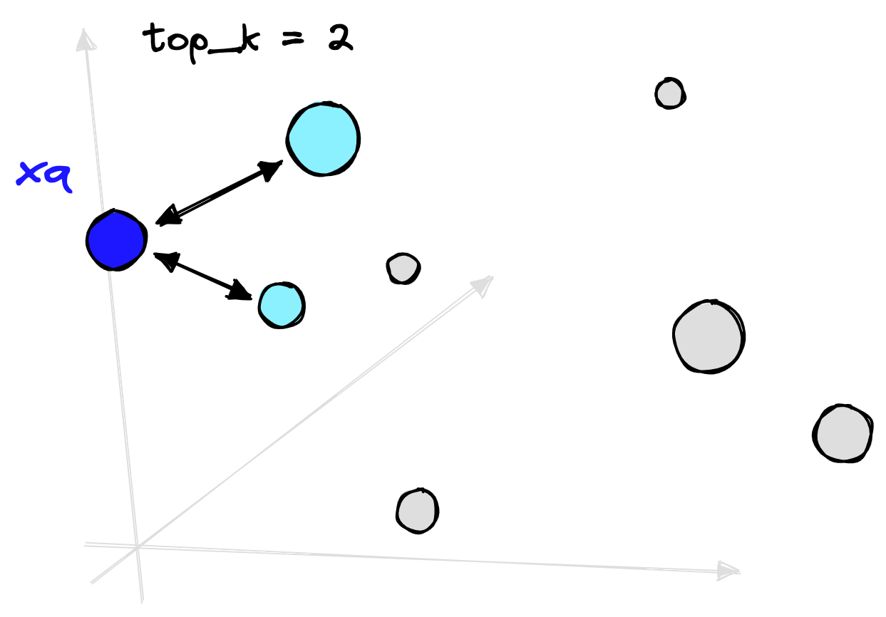
- Recall@k tells us if the correct answer is placed in the top _k_ positions.
- **M**ean **R**eciprocal **R**ank (MRR) calculates the average reciprocal rank of a correct answer.
We will implement a similar approach to in-batch evaluation. Using the sentence-transformers `RerankingEvaluator`, we can calculate the MRR score at the end of each training epoch using our evaluation data, `eval_pairs`.
Before initializing this evaluator, we need to remove duplicates from the eval data.
```json
{
"_key": "78c8e4046065",
"_type": "colabBlock",
"jsonContent": "{\n \"cells\": [\n {\n \"cell_type\": \"code\",\n \"execution_count\": 17,\n \"metadata\": {},\n \"outputs\": [\n {\n \"name\": \"stdout\",\n \"output_type\": \"stream\",\n \"text\": [\n \"1001 unique eval pairs\\n\"\n ]\n }\n ],\n \"source\": [\n \"dedup_eval_pairs = []\\n\",\n \"seen_eps = []\\n\",\n \"\\n\",\n \"for (query, episode) in eval_pairs:\\n\",\n \" if episode not in seen_eps:\\n\",\n \" seen_eps.append(episode)\\n\",\n \" dedup_eval_pairs.append((query, episode))\\n\",\n \"\\n\",\n \"eval_pairs = dedup_eval_pairs\\n\",\n \"print(f\\\"{len(eval_pairs)} unique eval pairs\\\")\"\n ]\n }\n ],\n \"metadata\": {\n \"environment\": {\n \"kernel\": \"python3\",\n \"name\": \"common-cu110.m91\",\n \"type\": \"gcloud\",\n \"uri\": \"gcr.io/deeplearning-platform-release/base-cu110:m91\"\n },\n \"interpreter\": {\n \"hash\": \"5188bc372fa413aa2565ae5d28228f50ad7b2c4ebb4a82c5900fd598adbb6408\"\n },\n \"kernelspec\": {\n \"display_name\": \"Python 3\",\n \"language\": \"python\",\n \"name\": \"python3\"\n },\n \"language_info\": {\n \"codemirror_mode\": {\n \"name\": \"ipython\",\n \"version\": 3\n },\n \"file_extension\": \".py\",\n \"mimetype\": \"text/x-python\",\n \"name\": \"python\",\n \"nbconvert_exporter\": \"python\",\n \"pygments_lexer\": \"ipython3\",\n \"version\": \"3.8.8\"\n }\n },\n \"nbformat\": 4,\n \"nbformat_minor\": 4\n}"
}
```
Then, we reformat the data into a list of dictionaries containing a query, its _positive_ episode (that it is paired with), and then all other episodes as _negatives_.
```python
from sentence_transformers.evaluation import RerankingEvaluator
# we must format samples into a list of:
# {'query': '', 'positive': [''], 'negative': []}
eval_set = []
eval_episodes = [pair[1] for pair in eval_pairs]
for i, (query, episode) in enumerate(eval_pairs):
negatives = eval_episodes[:i] + eval_episodes[i+1:]
eval_set.append(
{'query': query, 'positive': [episode], 'negative': negatives}
)
evaluator = RerankingEvaluator(eval_set, mrr_at_k=5, batch_size=batch_size)
```
We set the MRR@5 metric, meaning if the positive episode is returned within the top _five_ results, we return a positive score. Otherwise, the score would be zero.
---
_If the correct episode appeared at position_ __three_, the reciprocal rank of this sample would be calculated as 1/**3**. At position_ __one__ _we would return 1/**1**._
_As we’re calculating the_ **_mean_** _reciprocal rank, we take all sample scores and compute the mean, giving us our final MRR@5 score._
---
Using our evaluator, we first calculate the MRR@5 performance without any fine-tuning.
```json
{
"_key": "1f65e0420ad7",
"_type": "colabBlock",
"jsonContent": "{\n \"cells\": [\n {\n \"cell_type\": \"code\",\n \"execution_count\": 19,\n \"metadata\": {},\n \"outputs\": [\n {\n \"data\": {\n \"application/vnd.jupyter.widget-view+json\": {\n \"model_id\": \"2b320553075e41e3a94e072cedabc6e2\",\n \"version_major\": 2,\n \"version_minor\": 0\n },\n \"text/plain\": []\n },\n \"metadata\": {},\n \"output_type\": \"display_data\"\n },\n {\n \"data\": {\n \"text/plain\": [\n \"0.6827534406474566\"\n ]\n },\n \"execution_count\": 19,\n \"metadata\": {},\n \"output_type\": \"execute_result\"\n }\n ],\n \"source\": [\n \"evaluator(model, output_path='./')\"\n ]\n }\n ],\n \"metadata\": {\n \"environment\": {\n \"kernel\": \"python3\",\n \"name\": \"common-cu110.m91\",\n \"type\": \"gcloud\",\n \"uri\": \"gcr.io/deeplearning-platform-release/base-cu110:m91\"\n },\n \"interpreter\": {\n \"hash\": \"5188bc372fa413aa2565ae5d28228f50ad7b2c4ebb4a82c5900fd598adbb6408\"\n },\n \"kernelspec\": {\n \"display_name\": \"Python 3\",\n \"language\": \"python\",\n \"name\": \"python3\"\n },\n \"language_info\": {\n \"codemirror_mode\": {\n \"name\": \"ipython\",\n \"version\": 3\n },\n \"file_extension\": \".py\",\n \"mimetype\": \"text/x-python\",\n \"name\": \"python\",\n \"nbconvert_exporter\": \"python\",\n \"pygments_lexer\": \"ipython3\",\n \"version\": \"3.8.8\"\n }\n },\n \"nbformat\": 4,\n \"nbformat_minor\": 4\n}"
}
```
Returning an MRR@5 of _0.68_, we will compare this to the post-training MRR@5 score.
#### Fine-Tuning
With our evaluator ready, we can fine-tune our model. The Spotify article doesn’t give any information about the parameters they used, so we will stick with pretty typical training parameters for sentence transformer models using MNR loss. We train for a single epoch and _“warm up”_ the learning rate for the first 10% of training steps.
```json
{
"_key": "86d121db0d7c",
"_type": "colabBlock",
"jsonContent": "{\n \"cells\": [\n {\n \"cell_type\": \"code\",\n \"execution_count\": 20,\n \"metadata\": {},\n \"outputs\": [\n {\n \"data\": {\n \"application/vnd.jupyter.widget-view+json\": {\n \"model_id\": \"7921cd3990a54827bff2120183a93a5d\",\n \"version_major\": 2,\n \"version_minor\": 0\n },\n \"text/plain\": [\n \"100%|██████████| 1/1 [02:12:13<00:00]\"\n ]\n },\n \"metadata\": {},\n \"output_type\": \"display_data\"\n }\n ],\n \"source\": [\n \"epochs = 1\\n\",\n \"warmup_steps = int(len(loader) * epochs * 0.1)\\n\",\n \"\\n\",\n \"model.fit(\\n\",\n \" train_objectives=[(loader, loss)],\\n\",\n \" evaluator=evaluator,\\n\",\n \" epochs=epochs,\\n\",\n \" warmup_steps=warmup_steps,\\n\",\n \" output_path='distiluse-podcast-nq',\\n\",\n \" show_progress_bar=True\\n\",\n \")\"\n ]\n }\n ],\n \"metadata\": {\n \"environment\": {\n \"kernel\": \"python3\",\n \"name\": \"common-cu110.m91\",\n \"type\": \"gcloud\",\n \"uri\": \"gcr.io/deeplearning-platform-release/base-cu110:m91\"\n },\n \"interpreter\": {\n \"hash\": \"5188bc372fa413aa2565ae5d28228f50ad7b2c4ebb4a82c5900fd598adbb6408\"\n },\n \"kernelspec\": {\n \"display_name\": \"Python 3\",\n \"language\": \"python\",\n \"name\": \"python3\"\n },\n \"language_info\": {\n \"codemirror_mode\": {\n \"name\": \"ipython\",\n \"version\": 3\n },\n \"file_extension\": \".py\",\n \"mimetype\": \"text/x-python\",\n \"name\": \"python\",\n \"nbconvert_exporter\": \"python\",\n \"pygments_lexer\": \"ipython3\",\n \"version\": \"3.8.8\"\n }\n },\n \"nbformat\": 4,\n \"nbformat_minor\": 4\n}"
}
```
After fine-tuning, the model will be saved into the directory specified by `output_path`. In _distiluse-podcast-nq_, we will see all the required model files and a directory called _eval_. Here, we will find a post-training MRR@5 score of _0.89_, a sizeable 21-point improvement from the previous MRR@5 of _0.68_.
This score looks promising, but there’s further evaluation to be performed.
### Evaluation
We want to emulate a more _real-world_ scenario for the final evaluation step. Rather than calculating MRR@5 across small batches of data (as done previously), we should index _many_ episodes and recalculate some retrieval metrics.
Spotify details their _full-retrieval setting metrics_ as using Recall@30 and MRR@30, performed both on queries from the eval set and on their curated dataset.
Our eval set is small, so we can discard that. Instead, we will use the much larger test set `test_pairs`.
As before, we must deduplicate the episodes from the dataset.
```json
{
"_key": "f3c2d7926f46",
"_type": "colabBlock",
"jsonContent": "{\n \"cells\": [\n {\n \"cell_type\": \"code\",\n \"execution_count\": 22,\n \"metadata\": {},\n \"outputs\": [\n {\n \"name\": \"stdout\",\n \"output_type\": \"stream\",\n \"text\": [\n \"18579 unique test pairs\\n\"\n ]\n }\n ],\n \"source\": [\n \"dedup_test_pairs = []\\n\",\n \"seen_eps = []\\n\",\n \"\\n\",\n \"for (query, episode) in test_pairs:\\n\",\n \" if episode not in seen_eps:\\n\",\n \" seen_eps.append(episode)\\n\",\n \" dedup_test_pairs.append((query, episode))\\n\",\n \"\\n\",\n \"test_pairs = dedup_test_pairs\\n\",\n \"print(f\\\"{len(test_pairs)} unique test pairs\\\")\"\n ]\n }\n ],\n \"metadata\": {\n \"environment\": {\n \"kernel\": \"python3\",\n \"name\": \"common-cu110.m91\",\n \"type\": \"gcloud\",\n \"uri\": \"gcr.io/deeplearning-platform-release/base-cu110:m91\"\n },\n \"interpreter\": {\n \"hash\": \"5188bc372fa413aa2565ae5d28228f50ad7b2c4ebb4a82c5900fd598adbb6408\"\n },\n \"kernelspec\": {\n \"display_name\": \"Python 3\",\n \"language\": \"python\",\n \"name\": \"python3\"\n },\n \"language_info\": {\n \"codemirror_mode\": {\n \"name\": \"ipython\",\n \"version\": 3\n },\n \"file_extension\": \".py\",\n \"mimetype\": \"text/x-python\",\n \"name\": \"python\",\n \"nbconvert_exporter\": \"python\",\n \"pygments_lexer\": \"ipython3\",\n \"version\": \"3.8.8\"\n }\n },\n \"nbformat\": 4,\n \"nbformat_minor\": 4\n}"
}
```
This time, rather than keeping all of our embeddings stored in memory, we use a vector database, Pinecone.
We first [sign up for a free account](https://app.pinecone.io/), enter the default project and retrieve the _default_ API key.
Back in Python, we ensure the Pinecone client is installed with `pip install pinecone-client`. Then we initialize our connection to Pinecone and create a new vector index.
```python
import pinecone
pinecone.init(
api_key='YOUR_API_KEY', # app.pinecone.io
environment='YOUR_ENV' # find next to API key in console
)
# check if an evaluation index already exists, if not, create it
if 'evaluation' not in pinecone.list_indexes():
pinecone.create_index(
'evaluation', dimension=model.get_sentence_embedding_dimension(),
metric='cosine'
)
# now connect to the index
index = pinecone.Index('evaluation')
```
The vector index is where we will store all of our episode embeddings. We must encode the episode text using our fine-tuned `distiluse-podcast-nq` model and insert the embeddings into our index.
```python
to_upsert = []
queries = []
eps_batch = []
id_batch = []
upsert_batch = 64
for i, (query, episode) in enumerate(tqdm(test_pairs)):
# create batch
queries.append((query, str(i)))
eps_batch.append(episode)
id_batch.append(str(i))
# on reaching batch_size we encode and upsert
if len(eps_batch) == upsert_batch:
embeds = model.encode(eps_batch).tolist()
# insert to index
index.upsert(vectors=list(zip(id_batch, embeds)))
# refresh batch
eps_batch = []
id_batch = []
```
---
_Short on time? Download the fine-tuned model using_ _`model = SentenceTransformer('pinecone/distiluse-podcast-nq')`._
---
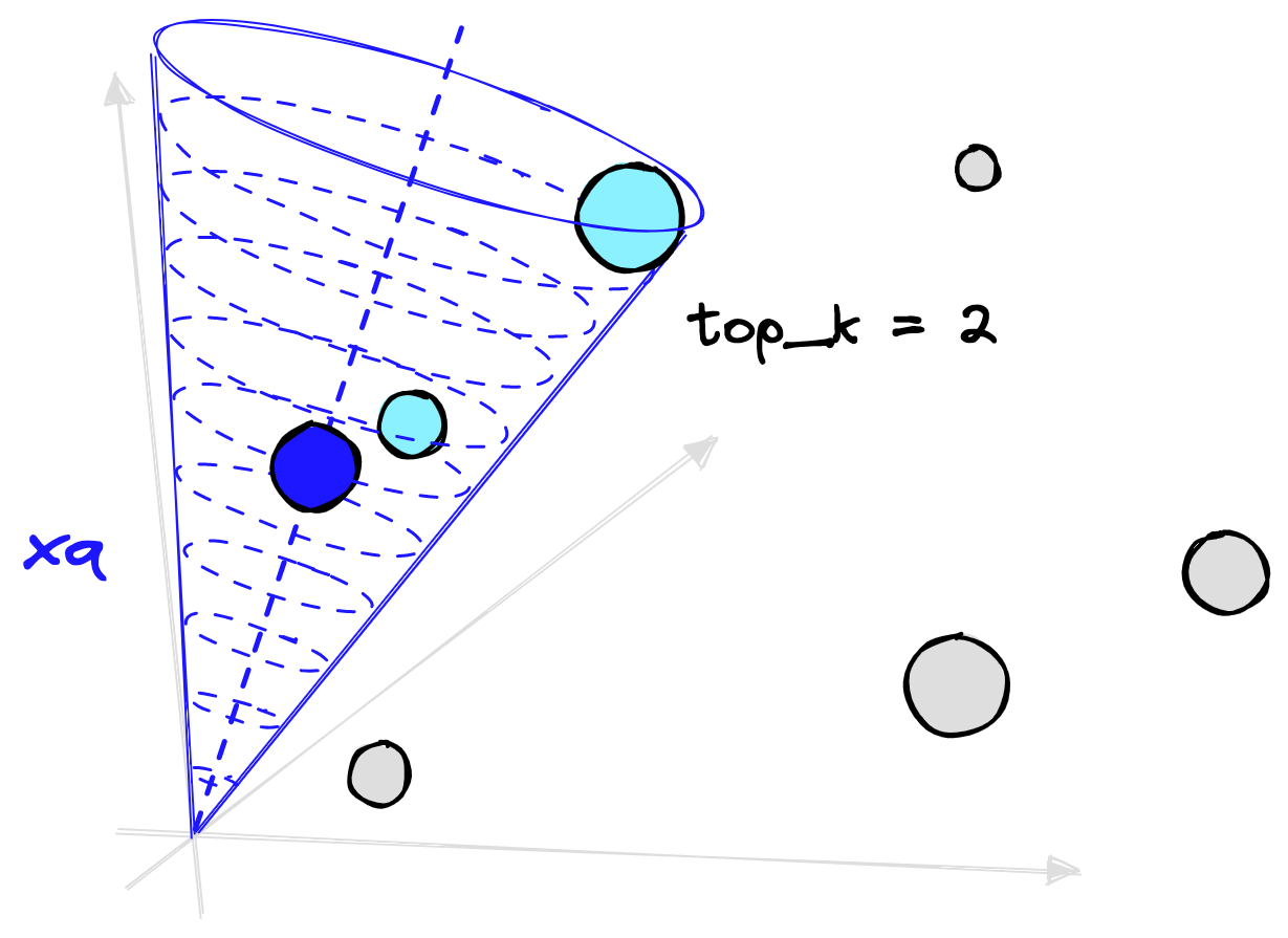
We will calculate the _Recall@K_ score, which differs slightly from the _MRR@K_ metric as if the match appears in the top K returned results, we score _1_; otherwise, we score _0_. As before, we take all query scores and compute the mean.
```json
{
"_key": "702885577823",
"_type": "colabBlock",
"jsonContent": "{\n \"cells\": [\n {\n \"cell_type\": \"code\",\n \"execution_count\": 24,\n \"metadata\": {},\n \"outputs\": [],\n \"source\": [\n \"recall_at_k = []\\n\",\n \"\\n\",\n \"for (query, i) in queries:\\n\",\n \" # encode the query to an embedding\\n\",\n \" xq = model.encode([query]).tolist()\\n\",\n \" res = index.query(xq, top_k=30)\\n\",\n \" # get IDs\\n\",\n \" ids = [x['id'] for x in res['results'][0]['matches']]\\n\",\n \" recall_at_k.append(1 if i in ids else 0)\"\n ]\n },\n {\n \"cell_type\": \"code\",\n \"execution_count\": 25,\n \"metadata\": {},\n \"outputs\": [\n {\n \"data\": {\n \"text/plain\": [\n \"0.883309112438775\"\n ]\n },\n \"execution_count\": 25,\n \"metadata\": {},\n \"output_type\": \"execute_result\"\n }\n ],\n \"source\": [\n \"sum(recall_at_k)/len(recall_at_k)\"\n ]\n }\n ],\n \"metadata\": {\n \"environment\": {\n \"kernel\": \"python3\",\n \"name\": \"common-cu110.m91\",\n \"type\": \"gcloud\",\n \"uri\": \"gcr.io/deeplearning-platform-release/base-cu110:m91\"\n },\n \"interpreter\": {\n \"hash\": \"5188bc372fa413aa2565ae5d28228f50ad7b2c4ebb4a82c5900fd598adbb6408\"\n },\n \"kernelspec\": {\n \"display_name\": \"Python 3\",\n \"language\": \"python\",\n \"name\": \"python3\"\n },\n \"language_info\": {\n \"codemirror_mode\": {\n \"name\": \"ipython\",\n \"version\": 3\n },\n \"file_extension\": \".py\",\n \"mimetype\": \"text/x-python\",\n \"name\": \"python\",\n \"nbconvert_exporter\": \"python\",\n \"pygments_lexer\": \"ipython3\",\n \"version\": \"3.8.8\"\n }\n },\n \"nbformat\": 4,\n \"nbformat_minor\": 4\n}"
}
```
So far, this looks great; 88% of the time, we are returning the exact positive episode within the top 30 results. But this does assume that our synthetic queries are perfect, which they are not.
We should measure model performance on more realistic queries, as Spotify did with their curated dataset. In this example, we have chosen a selection of episodes and manually written queries that fit the episode.
```python
curated = {
"funny show about after uni party house": 1,
"interview with cookbook author": 8,
"eat better during xmas holidays": 14,
"superhero film analysis": 27,
"how to tell more engaging stories": 33,
"how to make money with online content": 34,
"why is technology so addictive": 38
}
```
Using these curated samples, we returned a lower score of 0.57. Compared to 0.88, this seems low, but we must remember that there are likely other episodes that fit these queries. Meaning, we’re calculating recall assuming there are no other relevant queries.
What we can do is: measure this score against the score of the model before fine-tuning. We create a new Pinecone index and replicate the same steps but using the `distiluse-base-multilingual-cased-v2` sentence transformer. You can find the [full script here](https://github.com/pinecone-io/examples/blob/master/learn/search/semantic-search/spotify-podcast-search/spotify-podcast-search.ipynb).
Using this model, we return a score of just 0.29. By fine-tuning the model on this episode data, despite having no query pairs, we have improved episode retrieval performance by 28-points.
The technique we followed, informed by Spotify’s very own semantic search implementation, produced significant performance improvements.
Could this performance be better? Of course! Spotify fine-tuned their model using _three_ data sources. We can assume that the first two of those, pulled from Spotify’s past search logs, are of much higher quality than our synthetic dataset.
Merging the approach we have taken with a real dataset, as done by Spotify, is almost certain to produce a significantly higher-performing model.
The world of semantic search is already huge, but what is perhaps more exciting is the potential of this field. We will continue seeing new examples of semantic search, like Spotify’s podcast search, applied in many interesting and unique ways.
If you’re using Pinecone for semantic search and are interested in [showcasing your project](https://www.pinecone.io/community/), let us know! Comment them below or email them to us at [info@pinecone.io](mailto:info@pinecone.io).
## Resources
[Full Code Walkthrough](https://github.com/pinecone-io/examples/blob/master/learn/search/semantic-search/spotify-podcast-search/spotify-podcast-search.ipynb)
[1] [Podcast Content is Growing Audio Engagement](https://www.nielsen.com/us/en/insights/article/2020/podcast-content-is-growing-audio-engagement/) (2020), Nielsen
[2] S. Lebow, [Spotify Poised to Overtake Apple Podcasts This Year](https://www.emarketer.com/content/spotify-poised-overtake-apple-podcasts-this-year?ecid=NL1001) (2021), eMarketer
[3] A. Tamborrino [Introducing Natural Language Search for Podcast Episodes](https://engineering.atspotify.com/2022/03/introducing-natural-language-search-for-podcast-episodes/) (2022), Engineering at Spotify Blog
[4] O. Sharir, B. Peleg, Y. Shoham, [The Cost of Training NLP Models](https://arxiv.org/abs/2004.08900) (2020)
[5] N. Reimers, I. Gurevych, [Sentence-BERT: Sentence Embeddings using Siamese BERT-Networks](https://arxiv.org/abs/1908.10084) (2019), EMNLP